A Tutorial on Support Vector Machines for Pattern Recognition

Abstract. The tutorial starts with an overview of the concepts of VC dimension and structural risk minimization. We then describe linear Support Vector Machines (SVMs) for separable and non-separable data, working through a non-trivial example in detail. We describe a mechanical analogy, and discuss when SVM solutions are unique and when they are global. We describe how support vector training can be practically implemented, and discuss in detail the kernel mapping technique which is used to construct SVM solutions which are nonlinear in the data. We show how Support Vector machines can have very large (even infinite) VC dimension by computing the VC dimension for homogeneous polynomial and Gaussian radial basis function kernels. While very high VC dimension would normally bode ill for generalization performance, and while at present there exists no theory which shows that good generalization performance is guaranteed for SVMs, there are several arguments which support the observed high accuracy of SVMs, which we review. Results of some experiments which were inspired by these arguments are also presented. We give numerous examples and proofs of most of the key theorems. There is new material, and I hope that the reader will find that even old material is cast in a fresh light.

Keywords: support vector machines, statistical learning theory, VC dimension, pattern recognition

1. Introduction

The purpose of this paper is to provide an introductory yet extensive tutorial on the basic ideas behind Support Vector Machines (SVMs). The books (Vapnik, 1995; Vapnik, 1998) contain excellent descriptions of SVMs, but they leave room for an account whose purpose from the start is to teach. Although the subject can be said to have started in the late seventies (Vapnik, 1979), it is only now receiving increasing attention, and so the time appears suitable for an introductory review. The tutorial dwells entirely on the pattern recognition problem. Many of the ideas there carry directly over to the cases of regression estimation and linear operator inversion, but space constraints precluded the exploration of these topics here.

The tutorial contains some new material. All of the proofs are my own versions, where I have placed a strong emphasis on their being both clear and self-contained, to make the material as accessible as possible. This was done at the expense of some elegance and generality: however generality is usually easily added once the basic ideas are clear. The longer proofs are collected in the Appendix.

By way of motivation, and to alert the reader to some of the literature, we summarize some recent applications and extensions of support vector machines. For the pattern recognition case, SVMs have been used for isolated handwritten digit recognition (Cortes and Vapnik, 1995; Sch ̈olkopf, Burges and Vapnik, 1995; Sch ̈olkopf, Burges and Vapnik, 1996; Burges and Sch ̈olkopf, 1997), object recognition (Blanz et al., 1996), speaker identification (Schmidt, 1996), charmed quark detection1, face detection in images (Osuna, Freund and Girosi, 1997a), and text categorization (Joachims, 1997). For the regression estimation case, SVMs have been compared on benchmark time series prediction tests (M ̈uller et al., 1997; Mukherjee, Osuna and Girosi, 1997), the Boston housing problem (Drucker et al., 1997), and (on artificial data) on the PET operator inversion problem (Vapnik, Golowich and Smola, 1996). In most of these cases, SVM generalization performance (i.e. error rates on test sets) either matches or is significantly better than that of competing methods.

The use of SVMs for density estimation (Weston et al., 1997) and ANOVA decomposition (Stitson et al., 1997) has also been studied. Regarding extensions, the basic SVMs contain no prior knowledge of the problem (for example, a large class of SVMs for the image recognition problem would give the same results if the pixels were first permuted randomly (with each image suffering the same permutation), an act of vandalism that would leave the best performing neural networks severely handicapped) and much work has been done on incorporating prior knowledge into SVMs (Sch ̈olkopf, Burges and Vapnik, 1996; Sch ̈olkopf et al., 1998a; Burges, 1998). Although SVMs have good generalization performance, they can be abysmally slow in test phase, a problem addressed in (Burges, 1996; Osuna and Girosi, 1998). Recent work has generalized the basic ideas (Smola, Sch ̈olkopf and M ̈uller, 1998a; Smola and Sch ̈olkopf, 1998), shown connections to regularization theory (Smola, Sch ̈olkopf and M ̈uller, 1998b; Girosi, 1998; Wahba, 1998), and shown how SVM ideas can be incorporated in a wide range of other algorithms (Sch ̈olkopf, Smola and M ̈uller, 1998b; Sch ̈olkopf et al, 1998c). The reader may also find the thesis of (Sch ̈olkopf, 1997) helpful.

The problem which drove the initial development of SVMs occurs in several guises – the bias variance tradeoff (Geman and Bienenstock, 1992), capacity control (Guyon et al., 1992), overfitting (Montgomery and Peck, 1992) – but the basic idea is the same. Roughly speaking, for a given learning task, with a given finite amount of training data, the best generalization performance will be achieved if the right balance is struck between the accuracy attained on that particular training set, and the “capacity” of the machine, that is, the ability of the machine to learn any training set without error. A machine with too much capacity is like a botanist with a photographic memory who, when presented with a new tree, concludes that it is not a tree because it has a different number of leaves from anything she has seen before; a machine with too little capacity is like the botanist’s lazy brother, who declares that if it’s green, it’s a tree. Neither can generalize well. The exploration and formalization of these concepts has resulted in one of the shining peaks of the theory of statistical learning (Vapnik, 1979).

In the following, bold typeface will indicate vector or matrix quantities; normal typeface will be used for vector and matrix components and for scalars. We will label components of vectors and matrices with Greek indices, and label vectors and matrices themselves with Roman indices. Familiarity with the use of Lagrange multipliers to solve problems with equality or inequality constraints is assumed2.

2. A Bound on the Generalization Performance of a Pattern Recognition Learning Machine

There is a remarkable family of bounds governing the relation between the capacity of a learning machine and its performance3. The theory grew out of considerations of under what circumstances, and how quickly, the mean of some empirical quantity converges uniformly, as the number of data points increases, to the true mean (that which would be calculated from an infinite amount of data) (Vapnik, 1979). Let us start with one of these bounds.

The notation here will largely follow that of (Vapnik, 1995). Suppose we are given l observations. Each observation consists of a pair: a vector xi ∈ Rn, i = 1,…,l and the associated “truth” yi, given to us by a trusted source. In the tree recognition problem, xi might be a vector of pixel values (e.g. n = 256 for a 16×16 image), and yi would be 1 if the image contains a tree, and -1 otherwise (we use -1 here rather than 0 to simplify subsequent formulae). Now it is assumed that there exists some unknown probability distribution P(x, y) from which these data are drawn, i.e., the data are assumed “iid” (independently drawn and identically distributed). (We will use P for cumulative probability distributions, and p for their densities). Note that this assumption is more general than associating a fixed y with every x: it allows there to be a distribution of y for a given x. In that case, the trusted source would assign labels yi according to a fixed distribution, conditional on xi. However, after this Section, we will be assuming fixed y for given x.

Now suppose we have a machine whose task it is to learn the mapping xi “→ yi. The machine is actually defined by a set of possible mappings x “→ f(x, α), where the functions f(x, α) themselves are labeled by the adjustable parameters α. The machine is assumed to be deterministic: for a given input x, and choice of α, it will always give the same output f(x, α). A particular choice of α generates what we will call a “trained machine.” Thus, for example, a neural network with fixed architecture, with α corresponding to the weights and biases, is a learning machine in this sense.

The expectation of the test error for a trained machine is therefore: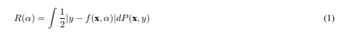Note that, when a density p(x, y) exists, dP(x, y) may be written p(x, y)dxdy. This is a nice way of writing the true mean error, but unless we have an estimate of what P(x, y) is, it is not very useful.

The quantity R(α) is called the expected risk, or just the risk. Here we will call it the actual risk, to emphasize that it is the quantity that we are ultimately interested in. The “empirical risk” Remp(α) is defined to be just the measured mean error rate on the training set (for a fixed, finite number of observations)4:Note that no probability distribution appears here. Remp(α) is a fixed number for a particular choice of α and for a particular training set {xi, yi}. The quantity 1/2 |yi − f(xi, α)| is called the loss. For the case described here, it can only take the values 0 and 1. Now choose some η such that 0 ≤ η ≤ 1. Then for losses taking these values, with probability 1 − η, the following bound holds (Vapnik, 1995):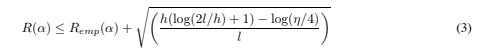where h is a non-negative integer called the Vapnik Chervonenkis (VC) dimension, and is a measure of the notion of capacity mentioned above. In the following we will call the right hand side of Eq. (3) the “risk bound.” We depart here from some previous nomenclature: the authors of (Guyon et al., 1992) call it the “guaranteed risk”, but this is something of a misnomer, since it is really a bound on a risk, not a risk, and it holds only with a certain probability, and so is not guaranteed. The second term on the right hand side is called the “VC confidence.”

We note three key points about this bound. First, remarkably, it is independent of P(x, y). It assumes only that both the training data and the test data are drawn independently according to some P(x, y). Second, it is usually not possible to compute the left hand side. Third, if we know h, we can easily compute the right hand side. Thus given several different learning machines (recall that “learning machine” is just another name for a family of functions f(x, α)), and choosing a fixed, sufficiently small η, by then taking that machine which minimizes the right hand side, we are choosing that machine which gives the lowest upper bound on the actual risk. This gives a principled method for choosing a learning machine for a given task, and is the essential idea of structural risk minimization (see Section 2.6).

Given a fixed family of learning machines to choose from, to the extent that the bound is tight for at least one of the machines, one will not be able to do better than this. To the extent that the bound is not tight for any, the hope is that the right hand side still gives useful information as to which learning machine minimizes the actual risk. The bound not being tight for the whole chosen family of learning machines gives critics a justifiable target at which to fire their complaints. At present, for this case, we must rely on experiment to be the judge.

2.1. The VC Dimension

The VC dimension is a property of a set of functions {f(α)} (again, we use α as a generic set of parameters: a choice of α specifies a particular function), and can be defined for various classes of function f. Here we will only consider functions that correspond to the two-class pattern recognition case, so that f(x, α) ∈ {−1, 1} ∀x, α. Now if a given set of l points can be labeled in all possible 2l ways, and for each labeling, a member of the set {f(α)} can be found which correctly assigns those labels, we say that that set of points is shattered by that set of functions. The VC dimension for the set of functions {f(α)} is defined as the maximum number of training points that can be shattered by {f(α)}. Note that, if the VC dimension is h, then there exists at least one set of h points that can be shattered, but it in general it will not be true that every set of h points can be shattered.

2.2. Shattering Points with Oriented Hyperplanes in Rη

Suppose that the space in which the data live is R2, and the set {f(α)} consists of oriented straight lines, so that for a given line, all points on one side are assigned the class 1, and all points on the other side, the class −1. The orientation is shown in Figure 1 by an arrow, specifying on which side of the line points are to be assigned the label 1. While it is possible to find three points that can be shattered by this set of functions, it is not possible to find four. Thus the VC dimension of the set of oriented lines in R2 is three.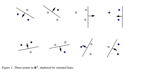Let’s now consider hyperplanes in Rn. The following theorem will prove useful (the proof is in the Appendix):

Theorem 1 Consider some set of m points in Rn. Choose any one of the points as origin. Then the m points can be shattered by oriented hyperplanes5 if and only if the position vectors of the remaining points are linearly independent6.

Corollary: The VC dimension of the set of oriented hyperplanes in Rn is n+ 1, since we can always choose n + 1 points, and then choose one of the points as origin, such that the position vectors of the remaining n points are linearly independent, but can never choose n + 2 such points (since no n + 1 vectors in Rn can be linearly independent). An alternative proof of the corollary can be found in (Anthony and Biggs, 1995), and references therein.

2.3. The VC Dimension and the Number of Parameters

The VC dimension thus gives concreteness to the notion of the capacity of a given set of functions. Intuitively, one might be led to expect that learning machines with many parameters would have high VC dimension, while learning machines with few parameters would have low VC dimension. There is a striking counterexample to this, due to E. Levin and J.S. Denker (Vapnik, 1995): A learning machine with just one parameter, but with infinite VC dimension (a family of classifiers is said to have infinite VC dimension if it can shatter l points, no matter how large l). Define the step function θ(x), x ∈ R : {θ(x) = 1 ∀x > 0; θ(x) = −1 ∀x ≤ 0}. Consider the one-parameter family of functions, defined byYou choose some number l, and present me with the task of finding l points that can be shattered. I choose them to be: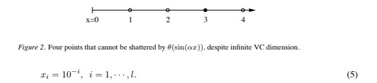You specify any labels you like:Then f(α) gives this labeling if I choose α to be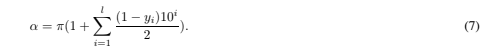Thus the VC dimension of this machine is infinite.

Interestingly, even though we can shatter an arbitrarily large number of points, we can also find just four points that cannot be shattered. They simply have to be equally spaced, and assigned labels as shown in Figure 2. This can be seen as follows: Write the phase at x1 as φ1 = 2nπ +δ. Then the choice of label y1 = 1 requires 0 < δ < π. The phase at x2, mod 2π, is 2δ; then y2 = 1 ⇒ 0 < δ < π/2. Similarly, point x3 forces δ > π/3. Then at x4, π/3 < δ < π/2 implies that f(x4, α) = −1, contrary to the assigned label. These four points are the analogy, for the set of functions in Eq. (4), of the set of three points lying along a line, for oriented hyperplanes in Rn. Neither set can be shattered by the chosen family of functions.

2.4. Minimizing The Bound by Minimizing h

Figure 3 shows how the second term on the right hand side of Eq. (3) varies with h, given a choice of 95% confidence level (η = 0.05) and assuming a training sample of size 10,000. The VC confidence is a monotonic increasing function of h. This will be true for any value of l.

Thus, given some selection of learning machines whose empirical risk is zero, one wants to choose that learning machine whose associated set of functions has minimal VC dimension. This will lead to a better upper bound on the actual error. In general, for non zero empirical risk, one wants to choose that learning machine which minimizes the right hand side of Eq. (3).

Note that in adopting this strategy, we are only using Eq. (3) as a guide. Eq. (3) gives (with some chosen probability) an upper bound on the actual risk. This does not prevent a particular machine with the same value for empirical risk, and whose function set has higher VC dimension, from having better performance. In fact an example of a system that gives good performance despite having infinite VC dimension is given in the next Section. Note also that the graph shows that for h/l > 0.37 (and for η = 0.05 and l = 10, 000), the VC confidence exceeds unity, and so for higher values the bound is guaranteed not tight.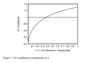

2.5. Two Examples

Consider the k’th nearest neighbour classifier, with k = 1. This set of functions has infinite VC dimension and zero empirical risk, since any number of points, labeled arbitrarily, will be successfully learned by the algorithm (provided no two points of opposite class lie right on top of each other). Thus the bound provides no information. In fact, for any classifier with infinite VC dimension, the bound is not even valid7. However, even though the bound is not valid, nearest neighbour classifiers can still perform well. Thus this first example is a cautionary tale: infinite “capacity” does not guarantee poor performance.

Let’s follow the time honoured tradition of understanding things by trying to break them, and see if we can come up with a classifier for which the bound is supposed to hold, but which violates the bound. We want the left hand side of Eq. (3) to be as large as possible, and the right hand side to be as small as possible. So we want a family of classifiers which gives the worst possible actual risk of 0.5, zero empirical risk up to some number of training observations, and whose VC dimension is easy to compute and is less than l (so that the bound is non trivial). An example is the following, which I call the “notebook classifier.” This classifier consists of a notebook with enough room to write down the classes of m training observations, where m ≤ l. For all subsequent patterns, the classifier simply says that all patterns have the same class. Suppose also that the data have as many positive (y = +1) as negative (y = −1) examples, and that the samples are chosen randomly. The notebook classifier will have zero empirical risk for up to m observations; 0.5 training error for all subsequent observations; 0.5 actual error, and VC dimension h = m. Substituting these values in Eq. (3), the bound becomes:which is certainly met for all η ifwhich is true, since f(z) is monotonic increasing, and f(z = 1) = 0.236.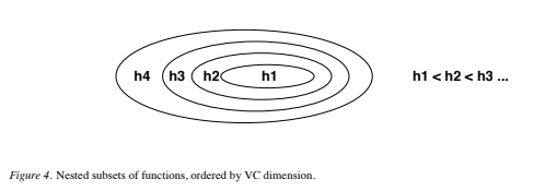

2.6. Structural Risk Minimization

We can now summarize the principle of structural risk minimization (SRM) (Vapnik, 1979). Note that the VC confidence term in Eq. (3) depends on the chosen class of functions, whereas the empirical risk and actual risk depend on the one particular function chosen by the training procedure. We would like to find that subset of the chosen set of functions, such that the risk bound for that subset is minimized. Clearly we cannot arrange things so that the VC dimension h varies smoothly, since it is an integer. Instead, introduce a “structure” by dividing the entire class of functions into nested subsets (Figure 4). For each subset, we must be able either to compute h, or to get a bound on h itself. SRM then consists of finding that subset of functions which minimizes the bound on the actual risk. This can be done by simply training a series of machines, one for each subset, where for a given subset the goal of training is simply to minimize the empirical risk. One then takes that trained machine in the series whose sum of empirical risk and VC confidence is minimal.

We have now laid the groundwork necessary to begin our exploration of support vector machines.

3. Linear Support Vector Machines

3.1. The Separable Case

We will start with the simplest case: linear machines trained on separable data (as we shall see, the analysis for the general case – nonlinear machines trained on non-separable data – results in a very similar quadratic programming problem). Again label the training data {xi, yi}, i = 1, ··· , l, yi ∈ {−1, 1}, xi ∈ Rd. Suppose we have some hyperplane which separates the positive from the negative examples (a “separating hyperplane”). The points x which lie on the hyperplane satisfy w · x + b = 0, where w is normal to the hyperplane, |b|/)w) is the perpendicular distance from the hyperplane to the origin, and )w) is the Euclidean norm of w. Let d+ (d−) be the shortest distance from the separating hyperplane to the closest positive (negative) example. Define the “margin” of a separating hyperplane to be d+ +d−. For the linearly separable case, the support vector algorithm simply looks for the separating hyperplane with largest margin. This can be formulated as follows: suppose that all the training data satisfy the following constraints:These can be combined into one set of inequalities:Now consider the points for which the equality in Eq. (10) holds (requiring that there exists such a point is equivalent to choosing a scale for w and b). These points lie on the hyperplane H1 : xi · w + b= 1 with normal w and perpendicular distance from the origin |1 − b|/)w). Similarly, the points for which the equality in Eq. (11) holds lie on the hyperplane H2 : xi · w + b = −1, with normal again w, and perpendicular distance from the origin | − 1 − b|/)w). Hence d+ = d− = 1/)w) and the margin is simply 2/)w). Note that H1 and H2 are parallel (they have the same normal) and that no training points fall between them. Thus we can find the pair of hyperplanes which gives the maximum margin by minimizing )w)2, subject to constraints (12).

Thus we expect the solution for a typical two dimensional case to have the form shown in Figure 5. Those training points for which the equality in Eq. (12) holds (i.e. those which wind up lying on one of the hyperplanes H1, H2), and whose removal would change the solution found, are called support vectors; they are indicated in Figure 5 by the extra circles.

We will now switch to a Lagrangian formulation of the problem. There are two reasons for doing this. The first is that the constraints (12) will be replaced by constraints on the Lagrange multipliers themselves, which will be much easier to handle. The second is that in this reformulation of the problem, the training data will only appear (in the actual training and test algorithms) in the form of dot products between vectors. This is a crucial property which will allow us to generalize the procedure to the nonlinear case (Section 4).

Thus, we introduce positive Lagrange multipliers αi, i = 1, ··· , l, one for each of the inequality constraints (12). Recall that the rule is that for constraints of the form ci ≥ 0, the constraint equations are multiplied by positive Lagrange multipliers and subtracted from the objective function, to form the Lagrangian. For equality constraints, the Lagrange multipliers are unconstrained. This gives Lagrangian: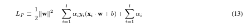We must now minimize LP with respect to w, b, and simultaneously require that the derivatives of LP with respect to all the αi vanish, all subject to the constraints αi ≥ 0 (let’s call this particular set of constraints C1). Now this is a convex quadratic programming problem, since the objective function is itself convex, and those points which satisfy the constraints also form a convex set (any linear constraint defines a convex set, and a set of N simultaneous linear constraints defines the intersection of N convex sets, which is also a convex set). This means that we can equivalently solve the following “dual” problem: maximize LP , subject to the constraints that the gradient of LP with respect to w and b vanish, and subject also to the constraints that the αi ≥ 0 (let’s call that particular set of constraints C2). This particular dual formulation of the problem is called the Wolfe dual (Fletcher, 1987). It has the property that the maximum of LP , subject to constraints C2, occurs at the same values of the w, b and α, as the minimum of LP , subject to constraints C18.

Requiring that the gradient of LP with respect to w and b vanish give the conditions: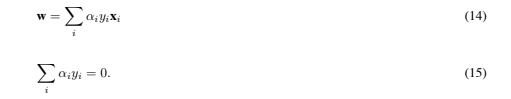Since these are equality constraints in the dual formulation, we can substitute them into Eq. (13) to give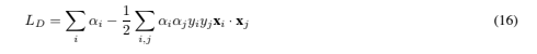Note that we have now given the Lagrangian different labels (P for primal, D for dual) to emphasize that the two formulations are different: LP and LD arise from the same objective function but with different constraints; and the solution is found by minimizing LP or by maximizing LD. Note also that if we formulate the problem with b = 0, which amounts to requiring that all hyperplanes contain the origin, the constraint (15) does not appear. This is a mild restriction for high dimensional spaces, since it amounts to reducing the number of degrees of freedom by one.

Support vector training (for the separable, linear case) therefore amounts to maximizing LD with respect to the αi, subject to constraints (15) and positivity of the αi, with solution given by (14). Notice that there is a Lagrange multiplier αi for every training point. In the solution, those points for which αi > 0 are called “support vectors”, and lie on one of the hyperplanes H1, H2. All other training points have αi = 0 and lie either on H1 or H2 (such that the equality in Eq. (12) holds), or on that side of H1 or H2 such that the strict inequality in Eq. (12) holds. For these machines, the support vectors are the critical elements of the training set. They lie closest to the decision boundary; if all other training points were removed (or moved around, but so as not to cross H1 or H2), and training was repeated, the same separating hyperplane would be found.

3.2. The Karush-Kuhn-Tucker Conditions

The Karush-Kuhn-Tucker (KKT) conditions play a central role in both the theory and practice of constrained optimization. For the primal problem above, the KKT conditions may be stated (Fletcher, 1987):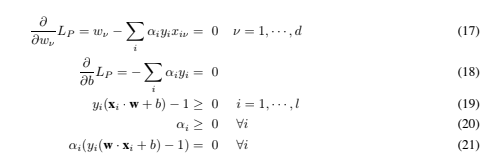The KKT conditions are satisfied at the solution of any constrained optimization problem (convex or not), with any kind of constraints, provided that the intersection of the set of feasible directions with the set of descent directions coincides with the intersection of the set of feasible directions for linearized constraints with the set of descent directions (see Fletcher, 1987; McCormick, 1983)). This rather technical regularity assumption holds for all support vector machines, since the constraints are always linear. Furthermore, the problem for SVMs is convex (a convex objective function, with constraints which give a convex feasible region), and for convex problems (if the regularity condition holds), the KKT conditions are necessary and sufficient for w, b, α to be a solution (Fletcher, 1987). Thus solving the SVM problem is equivalent to finding a solution to the KKT conditions. This fact results in several approaches to finding the solution (for example, the primal-dual path following method mentioned in Section 5).

As an immediate application, note that, while w is explicitly determined by the training procedure, the threshold b is not, although it is implicitly determined. However b is easily found by using the KKT “complementarity” condition, Eq. (21), by choosing any i for which αi += 0 and computing b (note that it is numerically safer to take the mean value of b resulting from all such equations).

Notice that all we’ve done so far is to cast the problem into an optimization problem where the constraints are rather more manageable than those in Eqs. (10), (11). Finding the solution for real world problems will usually require numerical methods. We will have more to say on this later. However, let’s first work out a rare case where the problem is nontrivial (the number of dimensions is arbitrary, and the solution certainly not obvious), but where the solution can be found analytically.

3.3. Optimal Hyperplanes: An Example

While the main aim of this Section is to explore a non-trivial pattern recognition problem where the support vector solution can be found analytically, the results derived here will also be useful in a later proof. For the problem considered, every training point will turn out to be a support vector, which is one reason we can find the solution analytically.

Consider n + 1 symmetrically placed points lying on a sphere Sn−1 of radius R: more precisely, the points form the vertices of an n-dimensional symmetric simplex. It is convenient to embed the points in Rn+1 in such a way that they all lie in the hyperplane which passes through the origin and which is perpendicular to the (n + 1)-vector (1, 1, …, 1) (in this formulation, the points lie on Sn−1, they span Rn, and are embedded in Rn+1). Explicitly, recalling that vectors themselves are labeled by Roman indices and their coordinates by Greek, the coordinates are given by: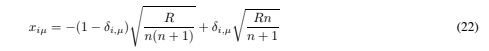where the Kronecker delta, δi,μ, is defined by δi,μ = 1 if μ = i, 0 otherwise. Thus, for example, the vectors for three equidistant points on the unit circle (see Figure 12) are: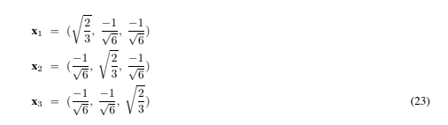One consequence of the symmetry is that the angle between any pair of vectors is the same (and is equal to arccos(−1/n)):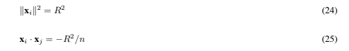or, more succinctly,Assigning a class label C ∈ {+1, −1} arbitrarily to each point, we wish to find that hyperplane which separates the two classes with widest margin. Thus we must maximize LD in Eq. (16), subject to αi ≥ 0 and also subject to the equality constraint, Eq. (15). Our strategy is to simply solve the problem as though there were no inequality constraints. If the resulting solution does in fact satisfy αi ≥ 0 ∀i, then we will have found the general solution, since the actual maximum of LD will then lie in the feasible region, provided the equality constraint, Eq. (15), is also met. In order to impose the equality constraint we introduce an additional Lagrange multiplier λ. Thus we seek to maximizewhere we have introduced the Hessian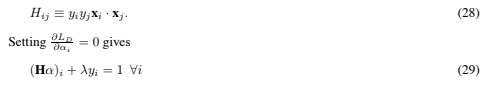Now H has a very simple structure: the off-diagonal elements are −yiyjR2/n, and the diagonal elements are R2. The fact that all the off-diagonal elements differ only by factors of yi suggests looking for a solution which has the form:where a and b are unknowns. Plugging this form in Eq. (29) gives:Thusand substituting this into the equality constraint Eq. (15) to find a, b giveswhich gives for the solutionAlso,Hence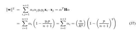Note that this is one of those cases where the Lagrange multiplier λ can remain undetermined (although determining it is trivial). We have now solved the problem, since all the αi are clearly positive or zero (in fact the αi will only be zero if all training points have the same class). Note that )w) depends only on the number of positive (negative) polarity points, and not on how the class labels are assigned to the points in Eq. (22). This is clearly not true of w itself, which is given byThe margin, M = 2/)w), is thus given byThus when the number of points n + 1 is even, the minimum margin occurs when p = 0 (equal numbers of positive and negative examples), in which case the margin is Mmin = 2R/√n. If n + 1 is odd, the minimum margin occurs when p = ±1, in which case Mmin = 2R(n + 1)/(n√n + 2). In both cases, the maximum margin is given by Mmax = R(n + 1)/n. Thus, for example, for the two dimensional simplex consisting of three points lying on S1 (and spanning R2), and with labeling such that not all three points have the same polarity, the maximum and minimum margin are both 3R/2 (see Figure (12)).

Note that the results of this Section amount to an alternative, constructive proof that the VC dimension of oriented separating hyperplanes in Rn is at least n + 1.

3.4. Test Phase

Once we have trained a Support Vector Machine, how can we use it? We simply determine on which side of the decision boundary (that hyperplane lying half way between H1 and H2 and parallel to them) a given test pattern x lies and assign the corresponding class label, i.e. we take the class of x to be sgn(w · x + b).

3.5. The Non-Separable Case

The above algorithm for separable data, when applied to non-separable data, will find no feasible solution: this will be evidenced by the objective function (i.e. the dual Lagrangian) growing arbitrarily large. So how can we extend these ideas to handle non-separable data? We would like to relax the constraints (10) and (11), but only when necessary, that is, we would like to introduce a further cost (i.e. an increase in the primal objective function) for doing so. This can be done by introducing positive slack variables ξi, i = 1, ··· , l in the constraints (Cortes and Vapnik, 1995), which then become: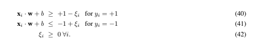Thus, for an error to occur, the corresponding ξi must exceed unity, so , i ξi is an upper bound on the number of training errors. Hence a natural way to assign an extra cost for errors is to change the objective function to be minimized from )w)2/2 to )w)2/2 +C (, i ξi)k, where C is a parameter to be chosen by the user, a larger C corresponding to assigning a higher penalty to errors. As it stands, this is a convex programming problem for any positive integer k; for k = 2 and k = 1 it is also a quadratic programming problem, and the choice k = 1 has the further advantage that neither the ξi, nor their Lagrange multipliers, appear in the Wolfe dual problem, which becomes:

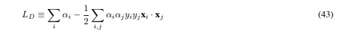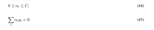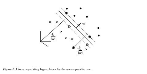
Maximize:subject to:The solution is again given by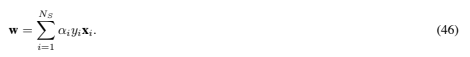where NS is the number of support vectors. Thus the only difference from the optimal hyperplane case is that the αi now have an upper bound of C. The situation is summarized schematically in Figure 6.

We will need the Karush-Kuhn-Tucker conditions for the primal problem. The primal Lagrangian is

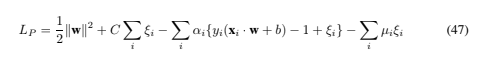
where the μi are the Lagrange multipliers introduced to enforce positivity of the ξi. The KKT conditions for the primal problem are therefore (note i runs from 1 to the number of training points, and ν from 1 to the dimension of the data)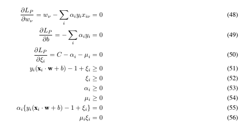As before, we can use the KKT complementarity conditions, Eqs. (55) and (56), to determine the threshold b. Note that Eq. (50) combined with Eq. (56) shows that ξi = 0 if αi < C. Thus we can simply take any training point for which 0 < αi < C to use Eq. (55) (with ξi = 0) to compute b. (As before, it is numerically wiser to take the average over all such training points.)

3.6. A Mechanical Analogy

Consider the case in which the data are in R2. Suppose that the i’th support vector exerts a force Fi = αiyiwˆ on a stiff sheet lying along the decision surface (the “decision sheet”) 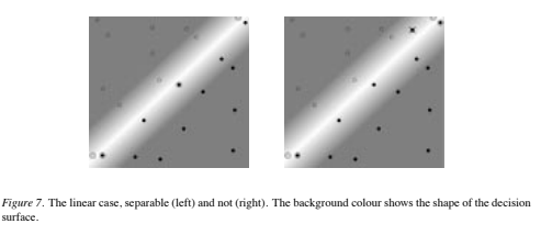(here wˆ denotes the unit vector in the direction w). Then the solution (46) satisfies the conditions of mechanical equilibrium:(Here the si are the support vectors, and ∧ denotes the vector product.) For data in Rn, clearly the condition that the sum of forces vanish is still met. One can easily show that the torque also vanishes.9

This mechanical analogy depends only on the form of the solution (46), and therefore holds for both the separable and the non-separable cases. In fact this analogy holds in general (i.e., also for the nonlinear case described below). The analogy emphasizes the interesting point that the “most important” data points are the support vectors with highest values of α, since they exert the highest forces on the decision sheet. For the non-separable case, the upper bound αi ≤ C corresponds to an upper bound on the force any given point is allowed to exert on the sheet. This analogy also provides a reason (as good as any other) to call these particular vectors “support vectors”10.

3.7. Examples by Pictures

Figure 7 shows two examples of a two-class pattern recognition problem, one separable and one not. The two classes are denoted by circles and disks respectively. Support vectors are identified with an extra circle. The error in the non-separable case is identified with a cross. The reader is invited to use Lucent’s SVM Applet (Burges, Knirsch and Haratsch, 1996) to experiment and create pictures like these (if possible, try using 16 or 24 bit color).

4. Nonlinear Support Vector Machines

How can the above methods be generalized to the case where the decision function11 is not a linear function of the data? (Boser, Guyon and Vapnik, 1992), showed that a rather old trick (Aizerman, 1964) can be used to accomplish this in an astonishingly straightforward way. First notice that the only way in which the data appears in the training problem, Eqs. (43) – (45), is in the form of dot products, xi · xj . Now suppose we first mapped the data to some other (possibly infinite dimensional) Euclidean space H, using a mapping which we will call Φ:Then of course the training algorithm would only depend on the data through dot products in H, i.e. on functions of the form Φ(xi)· Φ(xj ). Now if there were a “kernel function” K such that K(xi, xj ) = Φ(xi)·Φ(xj ), we would only need to use K in the training algorithm, and would never need to explicitly even know what Φ is. One example isIn this particular example, H is infinite dimensional, so it would not be very easy to work with Φ explicitly. However, if one replaces xi · xj by K(xi, xj ) everywhere in the training algorithm, the algorithm will happily produce a support vector machine which lives in an infinite dimensional space, and furthermore do so in roughly the same amount of time it would take to train on the un-mapped data. All the considerations of the previous sections hold, since we are still doing a linear separation, but in a different space.

But how can we use this machine? After all, we need w, and that will live in H also (see Eq. (46)). But in test phase an SVM is used by computing dot products of a given test point x with w, or more specifically by computing the sign ofwhere the si are the support vectors. So again we can avoid computing Φ(x) explicitly and use the K(si, x) = Φ(si) · Φ(x) instead.

Let us call the space in which the data live, L. (Here and below we use L as a mnemonic for “low dimensional”, and H for “high dimensional”: it is usually the case that the range of Φ is of much higher dimension than its domain). Note that, in addition to the fact that w lives in H, there will in general be no vector in L which maps, via the map Φ, to w. If there were, f(x) in Eq. (61) could be computed in one step, avoiding the sum (and making the corresponding SVM NS times faster, where NS is the number of support vectors). Despite this, ideas along these lines can be used to significantly speed up the test phase of SVMs (Burges, 1996). Note also that it is easy to find kernels (for example, kernels which are functions of the dot products of the xi in L) such that the training algorithm and solution found are independent of the dimension of both L and H.

In the next Section we will discuss which functions K are allowable and which are not. Let us end this Section with a very simple example of an allowed kernel, for which we can construct the mapping Φ.

Suppose that your data are vectors in R2, and you choose K(xi, xj )=(xi · xj )2. Then it’s easy to find a space H, and mapping Φ from R2 to H, such that (x · y)2 = Φ(x)· Φ(y): we choose H = R3 and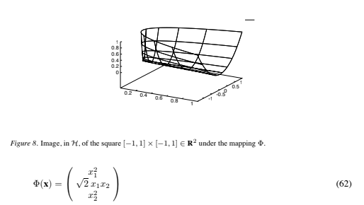

(note that here the subscripts refer to vector components). For data in L defined on the square [−1, 1] × [−1, 1] ∈ R2 (a typical situation, for grey level image data), the (entire) image of Φ is shown in Figure 8. This Figure also illustrates how to think of this mapping: the image of Φ may live in a space of very high dimension, but it is just a (possibly very contorted) surface whose intrinsic dimension12 is just that of L. Note that neither the mapping Φ nor the space H are unique for a given kernel. We could equally well have chosen H to again be R3 and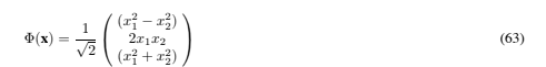or H to be R4 and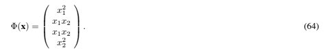The literature on SVMs usually refers to the space H as a Hilbert space, so let’s end this Section with a few notes on this point. You can think of a Hilbert space as a generalization of Euclidean space that behaves in a gentlemanly fashion. Specifically, it is any linear space, with an inner product defined, which is also complete with respect to the corresponding norm (that is, any Cauchy sequence of points converges to a point in the space). Some authors (e.g. (Kolmogorov, 1970)) also require that it be separable (that is, it must have a countable subset whose closure is the space itself), and some (e.g. Halmos, 1967) don’t. It’s a generalization mainly because its inner product can be any inner product, not just the scalar (“dot”) product used here (and in Euclidean spaces in general). It’s interesting that the older mathematical literature (e.g. Kolmogorov, 1970) also required that Hilbert spaces be infinite dimensional, and that mathematicians are quite happy defining infinite dimensional Euclidean spaces. Research on Hilbert spaces centers on operators in those spaces, since the basic properties have long since been worked out. Since some people understandably blanch at the mention of Hilbert spaces, I decided to use the term Euclidean throughout this tutorial.

4.1. Mercer’s Condition

For which kernels does there exist a pair {H, Φ}, with the properties described above, and for which does there not? The answer is given by Mercer’s condition (Vapnik, 1995; Courant and Hilbert, 1953): There exists a mapping Φ and an expansionif and only if, for any g(x) such that

thenNote that for specific cases, it may not be easy to check whether Mercer’s condition is satisfied. Eq. (67) must hold for every g with finite L2 norm (i.e. which satisfies Eq. (66)). However, we can easily prove that the condition is satisfied for positive integral powers of the dot product: K(x, y)=(x · y)p. We must show that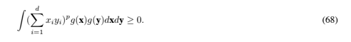The typical term in the multinomial expansion of (,di=1 xiyi)p contributes a term of the formto the left hand side of Eq. (67), which factorizes:One simple consequence is that any kernel which can be expressed as K(x, y) = ,∞p=0 cp(x·y)p, where the cp are positive real coefficients and the series is uniformly convergent, satisfies Mercer’s condition, a fact also noted in (Smola, Sch ̈olkopf and M ̈uller, 1998b).

Finally, what happens if one uses a kernel which does not satisfy Mercer’s condition? In general, there may exist data such that the Hessian is indefinite, and for which the quadratic programming problem will have no solution (the dual objective function can become arbitrarily large). However, even for kernels that do not satisfy Mercer’s condition, one might still find that a given training set results in a positive semidefinite Hessian, in which case the training will converge perfectly well. In this case, however, the geometrical interpretation described above is lacking.

4.2. Some Notes on Φ and H

Mercer’s condition tells us whether or not a prospective kernel is actually a dot product in some space, but it does not tell us how to construct Φ or even what H is. However, as with the homogeneous (that is, homogeneous in the dot product in L) quadratic polynomial kernel discussed above, we can explicitly construct the mapping for some kernels. In Section 6.1 we show how Eq. (62) can be extended to arbitrary homogeneous polynomial kernels, and that the corresponding space H is a Euclidean space of dimension 3d+p−1p4.

Thus for example, for a degree p = 4 polynomial, and for data consisting of 16 by 16 images (d=256), dim(H) is 183,181,376.

Usually, mapping your data to a “feature space” with an enormous number of dimensions would bode ill for the generalization performance of the resulting machine. After all, the set of all hyperplanes {w, b} are parameterized by dim(H) +1 numbers. Most pattern recognition systems with billions, or even an infinite, number of parameters would not make it past the start gate. How come SVMs do so well? One might argue that, given the form of solution, there are at most l + 1 adjustable parameters (where l is the number of training samples), but this seems to be begging the question13. It must be something to do with our requirement of maximum margin hyperplanes that is saving the day. As we shall see below, a strong case can be made for this claim.

Since the mapped surface is of intrinsic dimension dim(L), unless dim(L) = dim(H), it is obvious that the mapping cannot be onto (surjective). It also need not be one to one (bijective): consider x1 → −x1, x2 → −x2 in Eq. (62). The image of Φ need not itself be a vector space: again, considering the above simple quadratic example, the vector −Φ(x) is not in the image of Φ unless x = 0. Further, a little playing with the inhomogeneous kernelwill convince you that the corresponding Φ can map two vectors that are linearly dependent in L onto two vectors that are linearly independent in H.

So far we have considered cases where Φ is done implicitly. One can equally well turn things around and start with Φ, and then construct the corresponding kernel. For example (Vapnik, 1996), if L = R1, then a Fourier expansion in the data x, cut off after N terms, has the formand this can be viewed as a dot product between two vectors in R2N+1: a = ( aa/√a02 , a11,…,a21,…), and the mapped Φ(x)=( √12 , cos(x), cos(2x),…,sin(x),sin(2x),…). Then the corresponding (Dirichlet) kernel can be computed in closed form: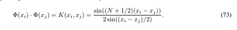This is easily seen as follows: letting δ ≡ xi − xj ,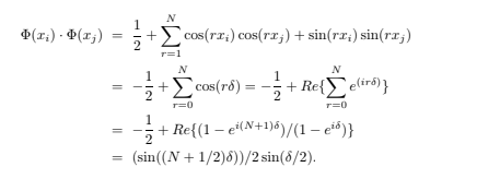Finally, it is clear that the above implicit mapping trick will work for any algorithm in which the data only appear as dot products (for example, the nearest neighbor algorithm). This fact has been used to derive a nonlinear version of principal component analysis by (Sch ̈olkopf, Smola and M ̈uller, 1998b); it seems likely that this trick will continue to find uses elsewhere.

4.3. Some Examples of Nonlinear SVMs

The first kernels investigated for the pattern recognition problem were the following:Eq. (74) results in a classifier that is a polynomial of degree p in the data; Eq. (75) gives a Gaussian radial basis function classifier, and Eq. (76) gives a particular kind of two-layer sigmoidal neural network. For the RBF case, the number of centers (NS in Eq. (61)), the centers themselves (the si), the weights (αi), and the threshold (b) are all produced automatically by the SVM training and give excellent results compared to classical RBFs, for the case of Gaussian RBFs (Sch ̈olkopf et al, 1997). For the neural network case, the first layer consists of NS sets of weights, each set consisting of dL (the dimension of the data) weights, and the second layer consists of NS weights (the αi), so that an evaluation simply requires taking a weighted sum of sigmoids, themselves evaluated on dot products 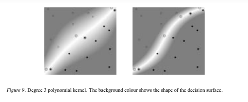of the test data with the support vectors. Thus for the neural network case, the architecture (number of weights) is determined by SVM training.

Note, however, that the hyperbolic tangent kernel only satisfies Mercer’s condition for certain values of the parameters κ and δ (and of the data )x)2). This was first noticed experimentally (Vapnik, 1995); however some necessary conditions on these parameters for positivity are now known14.

Figure 9 shows results for the same pattern recognition problem as that shown in Figure 7, but where the kernel was chosen to be a cubic polynomial. Notice that, even though the number of degrees of freedom is higher, for the linearly separable case (left panel), the solution is roughly linear, indicating that the capacity is being controlled; and that the linearly non-separable case (right panel) has become separable.

Finally, note that although the SVM classifiers described above are binary classifiers, they are easily combined to handle the multiclass case. A simple, effective combination trains N one-versus-rest classifiers (say, “one” positive, “rest” negative) for the N-class case and takes the class for a test point to be that corresponding to the largest positive distance (Boser, Guyon and Vapnik, 1992).

4.4. Global Solutions and Uniqueness

When is the solution to the support vector training problem global, and when is it unique? By “global”, we mean that there exists no other point in the feasible region at which the objective function takes a lower value. We will address two kinds of ways in which uniqueness may not hold: solutions for which {w, b} are themselves unique, but for which the expansion of w in Eq. (46) is not; and solutions whose {w, b} differ. Both are of interest: even if the pair {w, b} is unique, if the αi are not, there may be equivalent expansions of w which require fewer support vectors (a trivial example of this is given below), and which therefore require fewer instructions during test phase.

It turns out that every local solution is also global. This is a property of any convex programming problem (Fletcher, 1987). Furthermore, the solution is guaranteed to be unique if the objective function (Eq. (43)) is strictly convex, which in our case means that the Hessian must be positive definite (note that for quadratic objective functions F, the Hessian is positive definite if and only if F is strictly convex; this is not true for non-quadratic F: there, a positive definite Hessian implies a strictly convex objective function, but not vice versa (consider F = x4) (Fletcher, 1987)). However, even if the Hessian is positive semidefinite, the solution can still be unique: consider two points along the real line with coordinates x1 = 1 and x2 = 2, and with polarities + and −. Here the Hessian is positive semidefinite, but the solution (w = −2, b = 3, ξi = 0 in Eqs. (40), (41), (42)) is unique. It is also easy to find solutions which are not unique in the sense that the αi in the expansion of w are not unique:: for example, consider the problem of four separable points on a square in R2: x1 = [1, 1], x2 = [−1, 1], x3 = [−1, −1] and x4 = [1, −1], with polarities [+, −, −, +] respectively. One solution is w = [1, 0], b = 0, α = [0.25, 0.25, 0.25, 0.25]; another has the same w and b, but α = [0.5, 0.5, 0, 0] (note that both solutions satisfy the constraints αi > 0 and , i αiyi = 0). When can this occur in general? Given some solution α, choose an α& which is in the null space of the Hessian Hij = yiyjxi · xj , and require that α& be orthogonal to the vector all of whose components are 1. Then adding α& to α in Eq. (43) will leave LD unchanged. If 0 ≤ αi + α& i ≤ C and α& satisfies Eq. (45), then α + α& is also a solution15.

How about solutions where the {w, b} are themselves not unique? (We emphasize that this can only happen in principle if the Hessian is not positive definite, and even then, the solutions are necessarily global). The following very simple theorem shows that if non-unique solutions occur, then the solution at one optimal point is continuously deformable into the solution at the other optimal point, in such a way that all intermediate points are also solutions.

Theorem 2 Let the variable X stand for the pair of variables {w, b}. Let the Hessian for the problem be positive semidefinite, so that the objective function is convex. Let X0 and X1 be two points at which the objective function attains its minimal value. Then there exists a path X = X(τ ) = (1 − τ )X0 + τX1, τ ∈ [0, 1], such that X(τ ) is a solution for all τ .

Proof: Let the minimum value of the objective function be Fmin. Then by assumption, F(X0) = F(X1) = Fmin. By convexity of F, F(X(τ )) ≤ (1 − τ )F(X0) + τF(X1) = Fmin. Furthermore, by linearity, the X(τ ) satisfy the constraints Eq. (40), (41): explicitly (again combining both constraints into one):Although simple, this theorem is quite instructive. For example, one might think that the problems depicted in Figure 10 have several different optimal solutions (for the case of linear support vector machines). However, since one cannot smoothly move the hyperplane from one proposed solution to another without generating hyperplanes which are not solutions, we know that these proposed solutions are in fact not solutions at all. In fact, for each of these cases, the optimal unique solution is at w = 0, with a suitable choice of b (which has the effect of assigning the same label to all the points). Note that this is a perfectly 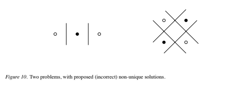acceptable solution to the classification problem: any proposed hyperplane (with w += 0) will cause the primal objective function to take a higher value. Finally, note that the fact that SVM training always finds a global solution is in contrast to the case of neural networks, where many local minima usually exist.

5. Methods of Solution

The support vector optimization problem can be solved analytically only when the number of training data is very small, or for the separable case when it is known beforehand which of the training data become support vectors (as in Sections 3.3 and 6.2). Note that this can happen when the problem has some symmetry (Section 3.3), but that it can also happen when it does not (Section 6.2). For the general analytic case, the worst case computational complexity is of order N3S (inversion of the Hessian), where NS is the number of support vectors, although the two examples given both have complexity of O(1).

However, in most real world cases, Equations (43) (with dot products replaced by kernels), (44), and (45) must be solved numerically. For small problems, any general purpose optimization package that solves linearly constrained convex quadratic programs will do. A good survey of the available solvers, and where to get them, can be found 16 in (Mor ́e and Wright, 1993).

For larger problems, a range of existing techniques can be brought to bear. A full exploration of the relative merits of these methods would fill another tutorial. Here we just describe the general issues, and for concreteness, give a brief explanation of the technique we currently use. Below, a “face” means a set of points lying on the boundary of the feasible region, and an “active constraint” is a constraint for which the equality holds. For more on nonlinear programming techniques see (Fletcher, 1987; Mangasarian, 1969; McCormick, 1983).

The basic recipe is to (1) note the optimality (KKT) conditions which the solution must satisfy, (2) define a strategy for approaching optimality by uniformly increasing the dual objective function subject to the constraints, and (3) decide on a decomposition algorithm so that only portions of the training data need be handled at a given time (Boser, Guyon and Vapnik, 1992; Osuna, Freund and Girosi, 1997a). We give a brief description of some of the issues involved. One can view the problem as requiring the solution of a sequence of equality constrained problems. A given equality constrained problem can be solved in one step by using the Newton method (although this requires storage for a factorization of the projected Hessian), or in at most l steps using conjugate gradient ascent (Press et al., 1992) (where l is the number of data points for the problem currently being solved: no extra storage is required). Some algorithms move within a given face until a new constraint is encountered, in which case the algorithm is restarted with the new constraint added to the list of equality constraints. This method has the disadvantage that only one new constraint is made active at a time. “Projection methods” have also been considered (Mor ́e, 1991), where a point outside the feasible region is computed, and then line searches and projections are done so that the actual move remains inside the feasible region. This approach can add several new constraints at once. Note that in both approaches, several active constraints can become inactive in one step. In all algorithms, only the essential part of the Hessian (the columns corresponding to αi += 0) need be computed (although some algorithms do compute the whole Hessian). For the Newton approach, one can also take advantage of the fact that the Hessian is positive semidefinite by diagonalizing it with the Bunch-Kaufman algorithm (Bunch and Kaufman, 1977; Bunch and Kaufman, 1980) (if the Hessian were indefinite, it could still be easily reduced to 2×2 block diagonal form with this algorithm).

In this algorithm, when a new constraint is made active or inactive, the factorization of the projected Hessian is easily updated (as opposed to recomputing the factorization from scratch). Finally, in interior point methods, the variables are essentially rescaled so as to always remain inside the feasible region. An example is the “LOQO” algorithm of (Vanderbei, 1994a; Vanderbei, 1994b), which is a primal-dual path following algorithm. This last method is likely to be useful for problems where the number of support vectors as a fraction of training sample size is expected to be large.

We briefly describe the core optimization method we currently use17. It is an active set method combining gradient and conjugate gradient ascent. Whenever the objective function is computed, so is the gradient, at very little extra cost. In phase 1, the search directions s are along the gradient. The nearest face along the search direction is found. If the dot product of the gradient there with s indicates that the maximum along s lies between the current point and the nearest face, the optimal point along the search direction is computed analytically (note that this does not require a line search), and phase 2 is entered. Otherwise, we jump to the new face and repeat phase 1. In phase 2, Polak-Ribiere conjugate gradient ascent (Press et al., 1992) is done, until a new face is encountered (in which case phase 1 is re-entered) or the stopping criterion is met. Note the following:

• Search directions are always projected so that the αi continue to satisfy the equality constraint Eq. (45). Note that the conjugate gradient algorithm will still work; we are simply searching in a subspace. However, it is important that this projection is implemented in such a way that not only is Eq. (45) met (easy), but also so that the angle between the resulting search direction, and the search direction prior to projection, is minimized (not quite so easy).
• We also use a “sticky faces” algorithm: whenever a given face is hit more than once, the search directions are adjusted so that all subsequent searches are done within that face. All “sticky faces” are reset (made “non-sticky”) when the rate of increase of the objective function falls below a threshold.
• The algorithm stops when the fractional rate of increase of the objective function F falls below a tolerance (typically 1e-10, for double precision). Note that one can also use as stopping criterion the condition that the size of the projected search direction falls below a threshold. However, this criterion does not handle scaling well.
• In my opinion the hardest thing to get right is handling precision problems correctly everywhere. If this is not done, the algorithm may not converge, or may be much slower than it needs to be.

A good way to check that your algorithm is working is to check that the solution satisfies all the Karush-Kuhn-Tucker conditions for the primal problem, since these are necessary and sufficient conditions that the solution be optimal. The KKT conditions are Eqs. (48) through (56), with dot products between data vectors replaced by kernels wherever they appear (note w must be expanded as in Eq. (48) first, since w is not in general the mapping of a point in L). Thus to check the KKT conditions, it is sufficient to check that the αi satisfy 0 ≤ αi ≤ C, that the equality constraint (49) holds, that all points for which 0 ≤ αi < C satisfy Eq. (51) with ξi = 0, and that all points with αi = C satisfy Eq. (51) for some ξi ≥ 0. These are sufficient conditions for all the KKT conditions to hold: note that by doing this we never have to explicitly compute the ξi or μi, although doing so is trivial.

5.1. Complexity, Scalability, and Parallelizability

Support vector machines have the following very striking property. Both training and test functions depend on the data only through the kernel functions K(xi, xj ). Even though it corresponds to a dot product in a space of dimension dH, where dH can be very large or infinite, the complexity of computing K can be far smaller. For example, for kernels of the form K = (xi · xj )p, a dot product in H would require of order 3dL+p−1p4 operations, whereas the computation of K(xi, xj ) requires only O(dL) operations (recall dL is the dimension of the data). It is this fact that allows us to construct hyperplanes in these very high dimensional spaces yet still be left with a tractable computation. Thus SVMs circumvent both forms of the “curse of dimensionality”: the proliferation of parameters causing intractable complexity, and the proliferation of parameters causing overfitting.

5.1.1. Training

For concreteness, we will give results for the computational complexity of one the the above training algorithms (Bunch-Kaufman)18 (Kaufman, 1998). These results assume that different strategies are used in different situations. We consider the problem of training on just one “chunk” (see below). Again let l be the number of training points, NS the number of support vectors (SVs), and dL the dimension of the input data.

In the case where most SVs are not at the upper bound, and NS/l << 1, the number of operations C is O(N3S + (N2S)l + NSdLl). If instead NS/l ≈ 1, then C is O(N3S + NSl + NSdLl) (basically by starting in the interior of the feasible region). For the case where most SVs are at the upper bound, and NS/l << 1, then C is O(N2S + NSdLl). Finally, if most SVs are at the upper bound, and NS/l ≈ 1, we have C of O(DLl2).

For larger problems, two decomposition algorithms have been proposed to date. In the “chunking” method (Boser, Guyon and Vapnik, 1992), one starts with a small, arbitrary subset of the data and trains on that. The rest of the training data is tested on the resulting classifier, and a list of the errors is constructed, sorted by how far on the wrong side of the  margin they lie (i.e. how egregiously the KKT conditions are violated). The next chunk is constructed from the first N of these, combined with the NS support vectors already found, where N + NS is decided heuristically (a chunk size that is allowed to grow too quickly or too slowly will result in slow overall convergence). Note that vectors can be dropped from a chunk, and that support vectors in one chunk may not appear in the final solution. This process is continued until all data points are found to satisfy the KKT conditions.

The above method requires that the number of support vectors NS be small enough so that a Hessian of size NS by NS will fit in memory. An alternative decomposition algorithm has been proposed which overcomes this limitation (Osuna, Freund and Girosi, 1997b). Again, in this algorithm, only a small portion of the training data is trained on at a given time, and furthermore, only a subset of the support vectors need be in the “working set” (i.e. that set of points whose α’s are allowed to vary). This method has been shown to be able to easily handle a problem with 110,000 training points and 100,000 support vectors. However, it must be noted that the speed of this approach relies on many of the support vectors having corresponding Lagrange multipliers αi at the upper bound, αi = C.

These training algorithms may take advantage of parallel processing in several ways. First, all elements of the Hessian itself can be computed simultaneously. Second, each element often requires the computation of dot products of training data, which could also be parallelized. Third, the computation of the objective function, or gradient, which is a speed bottleneck, can be parallelized (it requires a matrix multiplication). Finally, one can envision parallelizing at a higher level, for example by training on different chunks simultaneously. Schemes such as these, combined with the decomposition algorithm of (Osuna, Freund and Girosi, 1997b), will be needed to make very large problems (i.e. >> 100,000 support vectors, with many not at bound), tractable.

5.1.2. Testing

In test phase, one must simply evaluate Eq. (61), which will require O(MNS) operations, where M is the number of operations required to evaluate the kernel. For dot product and RBF kernels, M is O(dL), the dimension of the data vectors. Again, both the evaluation of the kernel and of the sum are highly parallelizable procedures. In the absence of parallel hardware, one can still speed up test phase by a large factor, as described in Section 9.

6. The VC Dimension of Support Vector Machines

We now show that the VC dimension of SVMs can be very large (even infinite). We will then explore several arguments as to why, in spite of this, SVMs usually exhibit good generalization performance. However it should be emphasized that these are essentially plausibility arguments. Currently there exists no theory which guarantees that a given family of SVMs will have high accuracy on a given problem.

We will call any kernel that satisfies Mercer’s condition a positive kernel, and the corresponding space H the embedding space. We will also call any embedding space with minimal dimension for a given kernel a “minimal embedding space”. We have the following

Theorem 3 Let K be a positive kernel which corresponds to a minimal embedding space H. Then the VC dimension of the corresponding support vector machine (where the error penalty C in Eq. (44) is allowed to take all values) is dim(H)+1.

Proof: If the minimal embedding space has dimension dH, then dH points in the image of L under the mapping Φ can be found whose position vectors in H are linearly independent. From Theorem 1, these vectors can be shattered by hyperplanes in H. Thus by either restricting ourselves to SVMs for the separable case (Section 3.1), or for which the error penalty C is allowed to take all values (so that, if the points are linearly separable, a C can be found such that the solution does indeed separate them), the family of support vector machines with kernel K can also shatter these points, and hence has VC dimension dH +1.

Let’s look at two examples.

6.1. The VC Dimension for Polynomial Kernels

Consider an SVM with homogeneous polynomial kernel, acting on data in RdL :As in the case when dL = 2 and the kernel is quadratic (Section 4), one can explicitly construct the map Φ. Letting zi = x1ix2i, so that K(x1, x2)=(z1 + ··· + zdL )p, we see that each dimension of H corresponds to a term with given powers of the zi in the expansion of K. In fact if we choose to label the components of Φ(x) in this manner, we can explicitly write the mapping for any p and dL:

This leads to

Theorem 4 If the space in which the data live has dimension dL (i.e. L = RdL ), the dimension of the minimal embedding space, for homogeneous polynomial kernels of degree p (K(x1, x2)=(x1 · x2)p, x1, x2 ∈ RdL ), is 3dL+p−1p4.

(The proof is in the Appendix). Thus the VC dimension of SVMs with these kernels is 3dL+p−1p4 + 1. As noted above, this gets very large very quickly.

6.2. The VC Dimension for Radial Basis Function Kernels

Theorem 5 Consider the class of Mercer kernels for which K(x1, x2) → 0 as )x1 − x2)→∞, and for which K(x, x)is O(1), and assume that the data can be chosen arbitrarily from Rd. Then the family of classifiers consisting of support vector machines using these kernels, and for which the error penalty is allowed to take all values, has infinite VC dimension.

Proof: The kernel matrix, Kij ≡ K(xi, xj ), is a Gram matrix (a matrix of dot products: see (Horn, 1985)) in H. Clearly we can choose training data such that all off-diagonal elements Ki’=j can be made arbitrarily small, and by assumption all diagonal elements Ki=j are of O(1). The matrix K is then of full rank; hence the set of vectors, whose dot products in H form K, are linearly independent (Horn, 1985); hence, by Theorem 1, the points can be shattered by hyperplanes in H, and hence also by support vector machines with sufficiently large error penalty. Since this is true for any finite number of points, the VC dimension of these classifiers is infinite.

Note that the assumptions in the theorem are stronger than necessary (they were chosen to make the connection to radial basis functions clear). In fact it is only necessary that l training points can be chosen such that the rank of the matrix Kij increases without limit as l increases. For example, for Gaussian RBF kernels, this can also be accomplished (even for training data restricted to lie in a bounded subset of RdL ) by choosing small enough RBF widths. However in general the VC dimension of SVM RBF classifiers can certainly be finite, and indeed, for data restricted to lie in a bounded subset of RdL , choosing restrictions on the RBF widths is a good way to control the VC dimension.

This case gives us a second opportunity to present a situation where the SVM solution can be computed analytically, which also amounts to a second, constructive proof of the Theorem. For concreteness we will take the case for Gaussian RBF kernels of the form K(x1, x2) = e−#x1−x2#2/2σ2. Let us choose training points such that the smallest distance between any pair of points is much larger than the width σ. Consider the decision function evaluated on the support vector sj :The sum on the right hand side will then be largely dominated by the term i = j; in fact the ratio of that term to the contribution from the rest of the sum can be made arbitrarily large by choosing the training points to be arbitrarily far apart. In order to find the SVM solution, we again assume for the moment that every training point becomes a support vector, and we work with SVMs for the separable case (Section 3.1) (the same argument will hold for SVMs for the non-separable case if C in Eq. (44) is allowed to take large enough values). Since all points are support vectors, the equalities in Eqs. (10), (11) will hold for them. Let there be N+ (N−) positive (negative) polarity points. We further assume that all positive (negative) polarity points have the same value α+ (α−) for their Lagrange multiplier. (We will know that this assumption is correct if it delivers a solution which satisfies all the KKT conditions and constraints). Then Eqs. (19), applied to all the training data, and the equality constraint Eq. (18), becomewhich are satisfied by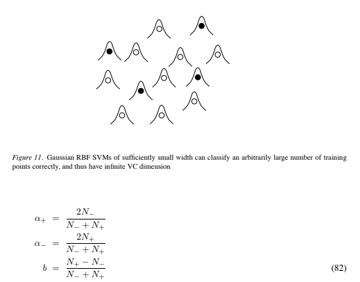Thus, since the resulting αi are also positive, all the KKT conditions and constraints are satisfied, and we must have found the global solution (with zero training errors). Since the number of training points, and their labeling, is arbitrary, and they are separated without error, the VC dimension is infinite.

The situation is summarized schematically in Figure 11.

Now we are left with a striking conundrum. Even though their VC dimension is infinite (if the data is allowed to take all values in RdL ), SVM RBFs can have excellent performance (Sch ̈olkopf et al, 1997). A similar story holds for polynomial SVMs. How come?

7. The Generalization Performance of SVMs

In this Section we collect various arguments and bounds relating to the generalization performance of SVMs. We start by presenting a family of SVM-like classifiers for which structural risk minimization can be rigorously implemented, and which will give us some insight as to why maximizing the margin is so important.

7.1. VC Dimension of Gap Tolerant Classifiers

Consider a family of classifiers (i.e. a set of functions Φ on Rd) which we will call “gap tolerant classifiers.” A particular classifier φ ∈ Φ is specified by the location and diameter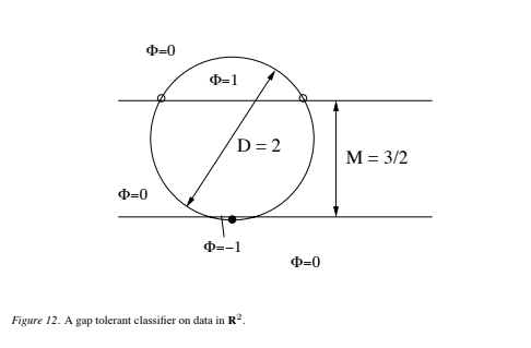of a ball in Rd, and by two hyperplanes, with parallel normals, also in Rd. Call the set of points lying between, but not on, the hyperplanes the “margin set.” The decision functions φ are defined as follows: points that lie inside the ball, but not in the margin set, are assigned class {±1}, depending on which side of the margin set they fall. All other points are simply defined to be “correct”, that is, they are not assigned a class by the classifier, and do not contribute to any risk. The situation is summarized, for d = 2, in Figure 12. This rather odd family of classifiers, together with a condition we will impose on how they are trained, will result in systems very similar to SVMs, and for which structural risk minimization can be demonstrated. A rigorous discussion is given in the Appendix.

Label the diameter of the ball D and the perpendicular distance between the two hyper-planes M. The VC dimension is defined as before to be the maximum number of points that can be shattered by the family, but by “shattered” we mean that the points can occur as errorsin all possible ways (see the Appendix for further discussion). Clearly we can control the VC dimension of a family of these classifiers by controlling the minimum margin M and maximum diameter D that members of the family are allowed to assume. For example, consider the family of gap tolerant classifiers in R2 with diameter D = 2, shown in Figure 12. Those with margin satisfying M ≤ 3/2 can shatter three points; if 3/2 < M < 2, they can shatter two; and if M ≥ 2, they can shatter only one. Each of these three families of classifiers corresponds to one of the sets of classifiers in Figure 4, with just three nested subsets of functions, and with h1 = 1, h2 = 2, and h3 = 3.

These ideas can be used to show how gap tolerant classifiers implement structural risk minimization. The extension of the above example to spaces of arbitrary dimension is encapsulated in a (modified) theorem of (Vapnik, 1995):

Theorem 6 For data in Rd, the VC dimension h of gap tolerant classifiers of minimum marginMmin and maximum diameter Dmax is bounded above19 by min{1D2 max/M2 min2, d}+1.

For the proof we assume the following lemma, which in (Vapnik, 1979) is held to follow from symmetry arguments20:

Lemma: Consider n ≤ d+ 1 points lying in a ball B ∈ Rd. Let the points be shatterable by gap tolerant classifiers with margin M. Then in order for M to be maximized, the points must lie on the vertices of an (n − 1)-dimensional symmetric simplex, and must also lie on the surface of the ball.

Proof: We need only consider the case where the number of points n satisfies n ≤ d + 1. (n>d+1 points will not be shatterable, since the VC dimension of oriented hyperplanes in Rd is d+ 1, and any distribution of points which can be shattered by a gap tolerant classifier can also be shattered by an oriented hyperplane; this also shows that h ≤ d + 1). Again we consider points on a sphere of diameter D, where the sphere itself is of dimension d−2. We will need two results from Section 3.3, namely (1) if n is even, we can find a distribution of n points (the vertices of the (n − 1)-dimensional symmetric simplex) which can be shattered by gap tolerant classifiers if D2max/M2min = n − 1, and (2) if n is odd, we can find a distribution of n points which can be so shattered if D2max/M2min = (n − 1)2(n + 1)/n2.

If n is even, at most n points can be shattered wheneverThus for n even the maximum number of points that can be shattered may be written 3D2max/M2min4 + 1. If n is odd, at most n points can be shattered when D2max/M2min = (n − 1)2(n + 1)/n2.

However, the quantity on the right hand side satisfiesfor all integer n > 1. Thus for n odd the largest number of points that can be shattered is certainly bounded above by 1D2max/M2min2 + 1, and from the above this bound is also satisfied when n is even. Hence in general the VC dimension h of gap tolerant classifiers must satisfyThis result, together with h ≤ d + 1, concludes the proof.

7.2. Gap Tolerant Classifiers, Structural Risk Minimization, and SVMs

Let’s see how we can do structural risk minimization with gap tolerant classifiers. We need only consider that subset of the Φ, call it ΦS, for which training “succeeds”, where by success we mean that all training data are assigned a label ∈ {±1} (note that these labels do not have to coincide with the actual labels, i.e. training errors are allowed). Within ΦS, find the subset which gives the fewest training errors – call this number of errors Nmin. Within that subset, find the function φ which gives maximum margin (and hence the lowest bound on the VC dimension). Note the value of the resulting risk bound (the right hand side of Eq. (3), using the bound on the VC dimension in place of the VC dimension). Next, within ΦS, find that subset which gives Nmin + 1 training errors. Again, within that subset, find the φ which gives the maximum margin, and note the corresponding risk bound. Iterate, and take that classifier which gives the overall minimum risk bound.

An alternative approach is to divide the functions Φ into nested subsets Φi, i ∈ Z, i ≥ 1, as follows: all φ ∈ Φi have {D, M} satisfying 1D2/M22 ≤ i. Thus the family of functions in Φi has VC dimension bounded above by min(i, d)+1. Note also that Φi ⊂ Φi+1. SRM then proceeds by taking that φ for which training succeeds in each subset and for which the empirical risk is minimized in that subset, and again, choosing that φ which gives the lowest overall risk bound.

Note that it is essential to these arguments that the bound (3) holds for any chosen decision function, not just the one that minimizes the empirical risk (otherwise eliminating solutions for which some training point x satisfies φ(x)=0 would invalidate the argument).

The resulting gap tolerant classifier is in fact a special kind of support vector machine which simply does not count data falling outside the sphere containing all the training data, or inside the separating margin, as an error. It seems very reasonable to conclude that support vector machines, which are trained with very similar objectives, also gain a similar kind of capacity control from their training. However, a gap tolerant classifier is not an SVM, and so the argument does not constitute a rigorous demonstration of structural risk minimization for SVMs. The original argument for structural risk minimization for SVMs is known to be flawed, since the structure there is determined by the data (see (Vapnik, 1995), Section 5.11). I believe that there is a further subtle problem with the original argument. The structure is defined so that no training points are members of the margin set. However, one must still specify how test points that fall into the margin are to be labeled. If one simply assigns the same, fixed class to them (say +1), then the VC dimension will be higher21 than the bound derived in Theorem 6. However, the same is true if one labels them all as errors (see the Appendix). If one labels them all as “correct”, one arrives at gap tolerant classifiers.

On the other hand, it is known how to do structural risk minimization for systems where the structure does depend on the data (Shawe-Taylor et al., 1996a; Shawe-Taylor et al., 1996b). Unfortunately the resulting bounds are much looser than the VC bounds above, which are already very loose (we will examine a typical case below where the VC bound is a factor of 100 higher than the measured test error). Thus at the moment structural risk minimization alone does not provide a rigorous explanation as to why SVMs often have good generalization performance. However, the above arguments strongly suggest that algorithms that minimize D2/M2 can be expected to give better generalization performance. Further evidence for this is found in the following theorem of (Vapnik, 1998), which we quote without proof22:

Theorem 7 For optimal hyperplanes passing through the origin, we havewhere P(error) is the probability of error on the test set, the expectation on the left is over all training sets of size l − 1, and the expectation on the right is over all training sets of size l.

However, in order for these observations to be useful for real problems, we need a way to compute the diameter of the minimal enclosing sphere described above, for any number of training points and for any kernel mapping.

7.3. How to Compute the Minimal Enclosing Sphere

Again let Φ be the mapping to the embedding space H. We wish to compute the radius of the smallest sphere in H which encloses the mapped training data: that is, we wish to minimize R2 subject towhere C ∈ H is the (unknown) center of the sphere. Thus introducing positive Lagrange multipliers λi, the primal Lagrangian isThis is again a convex quadratic programming problem, so we can instead maximize the Wolfe dual(where we have again replaced Φ(xi) · Φ(xj ) by K(xi, xj )) subject to:with solution given byThus the problem is very similar to that of support vector training, and in fact the code for the latter is easily modified to solve the above problem. Note that we were in a sense “lucky”, because the above analysis shows us that there exists an expansion (92) for the center; there is no a priori reason why we should expect that the center of the sphere in H should be expressible in terms of the mapped training data in this way. The same can be said of the solution for the support vector problem, Eq. (46). (Had we chosen some other geometrical construction, we might not have been so fortunate. Consider the smallest area equilateral triangle containing two given points in R2. If the points’ position vectors are linearly dependent, the center of the triangle cannot be expressed in terms of them.)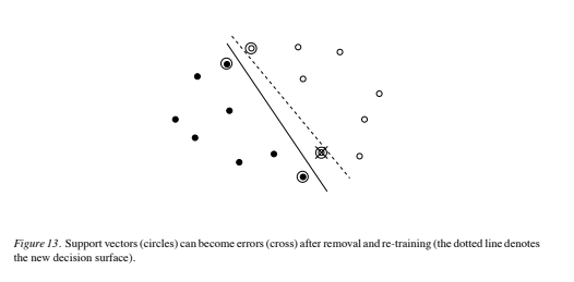

7.4. A Bound from Leave-One-Out

(Vapnik, 1995) gives an alternative bound on the actual risk of support vector machines:where P(error) is the actual risk for a machine trained on l − 1 examples, E[P(error)] is the expectation of the actual risk over all choices of training set of size l − 1, and E[Number of support vectors] is the expectation of the number of support vectors over all choices of training sets of size l. It’s easy to see how this bound arises: consider the typical situation after training on a given training set, shown in Figure 13.

We can get an estimate of the test error by removing one of the training points, re-training, and then testing on the removed point; and then repeating this, for all training points. From the support vector solution we know that removing any training points that are not support vectors (the latter include the errors) will have no effect on the hyperplane found. Thus the worst that can happen is that every support vector will become an error. Taking the expectation over all such training sets therefore gives an upper bound on the actual risk, for training sets of size l − 1.

Although elegant, I have yet to find a use for this bound. There seem to be many situations where the actual error increases even though the number of support vectors decreases, so the intuitive conclusion (systems that give fewer support vectors give better performance) often seems to fail. Furthermore, although the bound can be tighter than that found using the estimate of the VC dimension combined with Eq. (3), it can at the same time be less predictive, as we shall see in the next Section.

7.5. VC, SV Bounds and the Actual Risk

Let us put these observations to some use. As mentioned above, training an SVM RBF classifier will automatically give values for the RBF weights, number of centers, center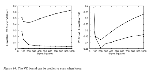positions, and threshold. For Gaussian RBFs, there is only one parameter left: the RBF width (σ in Eq. (80)) (we assume here only one RBF width for the problem). Can we find the optimal value for that too, by choosing that σ which minimizes D2/M2? Figure 14 shows a series of experiments done on 28×28 NIST digit data, with 10,000 training points and 60,000 test points. The top curve in the left hand panel shows the VC bound (i.e. the bound resulting from approximating the VC dimension in Eq. (3)23 by Eq. (85)), the middle curve shows the bound from leave-one-out (Eq. (93)), and the bottom curve shows the measured test error. Clearly, in this case, the bounds are very loose. The right hand panel shows just the VC bound (the top curve, for σ2 > 200), together with the test error, with the latter scaled up by a factor of 100 (note that the two curves cross). It is striking that the two curves have minima in the same place: thus in this case, the VC bound, although loose, seems to be nevertheless predictive. Experiments on digits 2 through 9 showed that the VC bound gave a minimum for which σ2 was within a factor of two of that which minimized the test error (digit 1 was inconclusive). Interestingly, in those cases the VC bound consistently gave a lower prediction for σ2 than that which minimized the test error. On the other hand, the leave-one-out bound, although tighter, does not seem to be predictive, since it had no minimum for the values of σ2 tested.

8. Limitations

Perhaps the biggest limitation of the support vector approach lies in choice of the kernel. Once the kernel is fixed, SVM classifiers have only one user-chosen parameter (the error penalty), but the kernel is a very big rug under which to sweep parameters. Some work has been done on limiting kernels using prior knowledge (Sch ̈olkopf et al., 1998a; Burges, 1998), but the best choice of kernel for a given problem is still a research issue.

A second limitation is speed and size, both in training and testing. While the speed problem in test phase is largely solved in (Burges, 1996), this still requires two training passes. Training for very large datasets (millions of support vectors) is an unsolved problem.

Discrete data presents another problem, although with suitable rescaling excellent results have nevertheless been obtained (Joachims, 1997). Finally, although some work has been done on training a multiclass SVM in one step24, the optimal design for multiclass SVM classifiers is a further area for research.

9. Extensions

We very briefly describe two of the simplest, and most effective, methods for improving the performance of SVMs.

The virtual support vector method (Sch ̈olkopf, Burges and Vapnik, 1996; Burges and Sch ̈olkopf, 1997), attempts to incorporate known invariances of the problem (for example, translation invariance for the image recognition problem) by first training a system, and then creating new data by distorting the resulting support vectors (translating them, in the case mentioned), and finally training a new system on the distorted (and the undistorted) data. The idea is easy to implement and seems to work better than other methods for incorporating invariances proposed so far.

The reduced set method (Burges, 1996; Burges and Sch ̈olkopf, 1997) was introduced to address the speed of support vector machines in test phase, and also starts with a trained SVM. The idea is to replace the sum in Eq. (46) by a similar sum, where instead of support vectors, computed vectors (which are not elements of the training set) are used, and instead of the αi, a different set of weights are computed. The number of parameters is chosen beforehand to give the speedup desired. The resulting vector is still a vector in H, and the parameters are found by minimizing the Euclidean norm of the difference between the original vector w and the approximation to it. The same technique could be used for SVM regression to find much more efficient function representations (which could be used, for example, in data compression).

Combining these two methods gave a factor of 50 speedup (while the error rate increased from 1.0% to 1.1%) on the NIST digits (Burges and Sch ̈olkopf, 1997).

10. Conclusions

SVMs provide a new approach to the problem of pattern recognition (together with regression estimation and linear operator inversion) with clear connections to the underlying statistical learning theory. They differ radically from comparable approaches such as neural networks: SVM training always finds a global minimum, and their simple geometric interpretation provides fertile ground for further investigation. An SVM is largely characterized by the choice of its kernel, and SVMs thus link the problems they are designed for with a large body of existing work on kernel based methods. I hope that this tutorial will encourage some to explore SVMs for themselves.

Acknowledgments

I’m very grateful to P. Knirsch, C. Nohl, E. Osuna, E. Rietman, B. Sch ̈olkopf, Y. Singer, A. Smola, C. Stenard, and V. Vapnik, for their comments on the manuscript. Thanks also to the reviewers, and to the Editor, U. Fayyad, for extensive, useful comments. Special thanks are due to V. Vapnik, under whose patient guidance I learned the ropes; to A. Smola and B. Sch ̈olkopf, for many interesting and fruitful discussions; and to J. Shawe-Taylor and D. Schuurmans, for valuable discussions on structural risk minimization.

Appendix

A.1. Proofs of Theorems

We collect here the theorems stated in the text, together with their proofs. The Lemma has a shorter proof using a “Theorem of the Alternative,” (Mangasarian, 1969) but we wished to keep the proofs as self-contained as possible.

Lemma 1 Two sets of points in Rn may be separated by a hyperplane if and only if the intersection of their convex hulls is empty.

Proof: We allow the notions of points in Rn, and position vectors of those points, to be used interchangeably in this proof. Let CA, CB be the convex hulls of two sets of points A, B in Rn. Let A − B denote the set of points whose position vectors are given by a − b, a ∈ A, b ∈ B (note that A − B does not contain the origin), and let CA − CB have the corresponding meaning for the convex hulls. Then showing that A and B are linearly separable (separable by a hyperplane) is equivalent to showing that the set A−B is linearly separable from the origin O. For suppose the latter: then ∃ w ∈ Rn, b ∈ R, b< 0 such that x · w + b > 0 ∀x ∈ A − B. Now pick some y ∈ B, and denote the set of all points a − b+ y, a ∈ A, b ∈ B by A − B + y. Then x · w + b > y · w ∀x ∈ A − B + y, and clearly y · w + b < y · w, so the sets A − B + y and y are linearly separable. Repeating this process shows that A − B is linearly separable from the origin if and only if A and B are linearly separable.

We now show that, if CA5 CB = ∅, then CA − CB is linearly separable from the origin. Clearly CA − CB does not contain the origin. Furthermore CA − CB is convex, since ∀x1 = a1 − b1, x2 = a2 − b2, λ ∈ [0, 1], a1, a2 ∈ CA, b1, b2 ∈ CB, we have (1−λ)x1+λx2 = ((1−λ)a1+λa2)−((1−λ)b1+λb2) ∈ CA −CB. Hence it is sufficient to show that any convex set S, which does not contain O, is linearly separable from O.  Let xmin ∈ S be that point whose Euclidean distance from O, )xmin), is minimal. (Note there can be only one such point, since if there were two, the chord joining them, which also lies in S, would contain points closer to O.) We will show that ∀x ∈ S, x · xmin > 0. Suppose ∃ x ∈ S such that x · xmin ≤ 0. Let L be the line segment joining xmin and x. Then convexity implies that L ⊂ S. Thus O /∈ L, since by assumption O /∈ S. Hence the three points O, x and xmin form an obtuse (or right) triangle, with obtuse (or right) angle occurring at the point O. Define nˆ ≡ (x − xmin)/)x − xmin). Then the distance from the closest point in L to O is )xmin)2 − (xmin · nˆ)2, which is less than )xmin)2. Hence x · xmin > 0 and S is linearly separable from O. Thus CA − CB is linearly separable from O, and a fortiori A − B is linearly separable from O, and thus A is linearly separable from B.

It remains to show that, if the two sets of points A, B are linearly separable, the intersection of their convex hulls if empty. By assumption there exists a pair w ∈ Rn, b ∈ R, such that ∀ai ∈ A, w·ai+b > 0 and ∀bi ∈ B, w·bi+b < 0. Consider a general point x ∈ CA. It may be written x = , i λiai, ,λi = 1, 0 ≤ λi ≤ 1. Then w· b+b = , i λi{w· ai +b} > 0.

Similarly, for points y ∈ CB, w · y + b < 0. Hence CA5 CB = ∅, since otherwise we would be able to find a point x = y which simultaneously satisfies both inequalities.

Theorem 1: Consider some set of m points in Rn. Choose any one of the points as origin. Then the m points can be shattered by oriented hyperplanes if and only if the position vectors of the remaining points are linearly independent.

Proof: Label the origin O, and assume that the m − 1 position vectors of the remaining points are linearly independent. Consider any partition of the m points into two subsets, S1 and S2, of order m1 and m2 respectively, so that m1 + m2 = m. Let S1 be the subset containing O. Then the convex hull C1 of S1 is that set of points whose position vectors x satisfywhere the s1i are the position vectors of the m1 points in S1 (including the null position vector of the origin). Similarly, the convex hull C2 of S2 is that set of points whose position vectors x satisfywhere the s2i are the position vectors of the m2 points in S2. Now suppose that C1 and C2 intersect. Then there exists an x ∈ Rn which simultaneously satisfies Eq. (A.1) and Eq. (A.2). Subtracting these equations gives a linear combination of the m − 1 non-null position vectors which vanishes, which contradicts the assumption of linear independence. By the lemma, since C1 and C2 do not intersect, there exists a hyperplane separating S1 and S2. Since this is true for any choice of partition, the m points can be shattered.

It remains to show that if the m−1 non-null position vectors are not linearly independent, then the m points cannot be shattered by oriented hyperplanes. If the m−1 position vectors are not linearly independent, then there exist m − 1 numbers, γi, such thatIf all the γi are of the same sign, then we can scale them so that γi ∈ [0, 1] and , i γi = 1. Eq. (A.3) then states that the origin lies in the convex hull of the remaining points; hence, by the lemma, the origin cannot be separated from the remaining points by a hyperplane, and the points cannot be shattered.

If the γi are not all of the same sign, place all the terms with negative γi on the right:where I1, I2 are the indices of the corresponding partition of S\O (i.e. of the set S with the origin removed). Now scale this equation so that either , j∈I1 , |γj | = 1 and k∈I2 |γk| ≤ 1, or , j∈I1 |γj | ≤ 1 and , k∈I2 |γk| = 1. Suppose without loss of generality that the latter holds. Then the left hand side of Eq. (A.4) is the position vector of a point lying in the convex hull of the points {6j∈I1 sj} 6 O (or, if the equality holds, of the points {6j∈I1 sj}), and the right hand side is the position vector of a point lying in the convex hull of the points 6 k∈I2 sk, so the convex hulls overlap, and by the lemma, the two sets of points cannot be separated by a hyperplane. Thus the m points cannot be shattered.

Theorem 4: If the data is d-dimensional (i.e. L = Rd), the dimension of the minimal embedding space, for homogeneous polynomial kernels of degree p (K(x1, x2)=(x1 · x2)p, x1, x2 ∈ Rd), is 3d+p−1p4.

Proof: First we show that the the number of components of Φ(x) is 3p+d−1p4. Label the components of Φ as in Eq. (79). Then a component is uniquely identified by the choice of the d integers ri ≥ 0, ,di=1 ri = p. Now consider p objects distributed amongst d − 1 partitions (numbered 1 through d − 1), such that objects are allowed to be to the left of all partitions, or to the right of all partitions. Suppose m objects fall between partitions q and q + 1. Let this correspond to a term xmq+1 in the product in Eq. (79). Similarly, m objects falling to the left of all partitions corresponds to a term xm1 , and m objects falling to the right of all partitions corresponds to a term xmd . Thus the number of distinct terms of the form xr1 1 xr2 2 ··· xrdd , ,di=1 ri = p, ri ≥ 0 is the number of way of distributing the objects and partitions amongst themselves, modulo permutations of the partitions and permutations of the objects, which is 3p+d−1p4.

Next we must show that the set of vectors with components Φr1r2···rd (x)span the space H. This follows from the fact that the components of Φ(x) are linearly independent functions. For suppose instead that the image of Φ acting on x ∈ L is a subspace of H. Then there exists a fixed nonzero vector V ∈ H such that Using the labeling introduced above, consider a particular component of Φ:Since Eq. (A.5) holds for all x, and since the mapping Φ in Eq. (79) certainly has all derivatives defined, we can apply the operator to Eq. (A.5), which will pick that one term with corresponding powers of the xi in Eq. (79), givingSince this is true for all choices of r1, ··· , rd such that,d i=1 ri = p, every component of V must vanish. Hence the image of Φ acting on x ∈ L spans H.

A.2. Gap Tolerant Classifiers and VC Bounds

The following point is central to the argument. One normally thinks of a collection of points as being “shattered” by a set of functions, if for any choice of labels for the points, a function from the set can be found which assigns those labels to the points. The VC dimension of that set of functions is then defined as the maximum number of points that can be so shattered. However, consider a slightly different definition. Let a set of points be shattered by a set of functions if for any choice of labels for the points, a function from the set can be found which assigns the incorrect labels to all the points. Again let the VC dimension of that set of functions be defined as the maximum number of points that can be so shattered.

It is in fact this second definition (which we adopt from here on) that enters the VC bound proofs (Vapnik, 1979; Devroye, Gy ̈orfi and Lugosi, 1996). Of course for functions whose range is {±1} (i.e. all data will be assigned either positive or negative class), the two definitions are the same. However, if all points falling in some region are simply deemed to be “errors”, or “correct”, the two definitions are different. As a concrete example, suppose we define “gap intolerant classifiers”, which are like gap tolerant classifiers, but which label all points lying in the margin or outside the sphere as errors. Consider again the situation in Figure 12, but assign positive class to all three points. Then a gap intolerant classifier with margin width greater than the ball diameter cannot shatter the points if we use the first definition of “shatter”, but can shatter the points if we use the second (correct) definition. With this caveat in mind, we now outline how the VC bounds can apply to functions with range {±1, 0}, where the label 0 means that the point is labeled “correct.” (The bounds will also apply to functions where 0 is defined to mean “error”, but the corresponding VC dimension will be higher, weakening the bound, and in our case, making it useless). We will follow the notation of (Devroye, Gy ̈orfi and Lugosi, 1996).

Consider points x ∈ Rd, and let p(x) denote a density on Rd. Let φ be a function on Rd with range {±1, 0}, and let Φ be a set of such functions. Let each x have an associated label yx ∈ {±1}. Let {x1, ··· , xn} be any finite number of points in Rd: then we require Φ to have the property that there exists at least one φ ∈ Φ such that φ(xi) ∈ {±1} ∀ xi.

For given φ, define the set of points A byWe require that the φ be such that all sets A are measurable. Let A denote the set of all A.

Definition: Let xi, i = 1, ··· , n be n points. We define the empirical risk for the set {xi, φ} to bewhere I is the indicator function. Note that the empirical risk is zero if φ(xi)=0 ∀ xi.

Definition: We define the actual risk for the function φ to beNote also that those points x for which φ(x)=0 do not contribute to the actual risk.

Definition: For fixed (x1, ··· , xn) ∈ Rd, let NA be the number of different sets inwhere the sets A are defined above. The n-th shatter coefficient of A is definedWe also define the VC dimension for the class A to be the maximum integer k ≥ 1 for which s(A, k)=2k.

Theorem 8 (adapted from Devroye, Gyorfi and Lugosi, 1996, Theorem 12.6):Given ̈ νn({xi, φ}), ν(φ) and s(A, n) defined above, and given n points (x1, …, xn) ∈ Rd, let Φ& denote that subset of Φ such that all φ ∈ Φ& satisfy φ(xi) ∈ {±1} ∀ xi. (This restriction may be viewed as part of the training algorithm). Then for any such φ,The proof is exactly that of (Devroye, Gy ̈orfi and Lugosi, 1996), Sections 12.3, 12.4 and 12.5, Theorems 12.5 and 12.6. We have dropped the “sup” to emphasize that this holds for any of the functions φ. In particular, it holds for those φ which minimize the empirical error and for which all training data take the values {±1}. Note however that the proof only holds for the second definition of shattering given above. Finally, note that the usual form of the VC bounds is easily derived from Eq. (A.14) by using s(A, n) ≤ (en/h)h (where h is the VC dimension) (Vapnik, 1995), setting η = 8s(A, n) exp−n‘2/32, and solving for 0.

Clearly these results apply to our gap tolerant classifiers of Section 7.1. For them, a particular classifier φ ∈ Φ is specified by a set of parameters {B, H, M}, where B is a ball in Rd, D ∈ R is the diameter of B, H is a d − 1 dimensional oriented hyperplane in Rd, and M ∈ R is a scalar which we have called the margin. H itself is specified by its normal (whose direction specifies which points H+ (H−) are labeled positive (negative) by the function), and by the minimal distance from H to the origin. For a given φ ∈ Φ, the margin set SM is defined as the set consisting of those points whose minimal distance to H is less than M/2. Define Z ≡ S ̄M5 B, Z+ ≡ Z 5 H+, and Z− ≡ Z 5 H−. The function φ is then defined as follows:and the corresponding sets A as in Eq. (A.9).

Notes

1. K. M ̈uller, Private Communication
2. The reader in whom this elicits a sinking feeling is urged to study (Strang, 1986; Fletcher, 1987; Bishop, 1995). There is a simple geometrical interpretation of Lagrange multipliers: at a boundary corresponding to a single constraint, the gradient of the function being extremized must be parallel to the gradient of the function whose contours specify the boundary. At a boundary corresponding to the intersection of constraints, the gradient must be parallel to a linear combination (non-negative in the case of inequality constraints) of the gradients of the functions whose contours specify the boundary.
3. In this paper, the phrase “learning machine” will be used for any function estimation algorithm, “training” for the parameter estimation procedure, “testing” for the computation of the function value, and “performance” for the generalization accuracy (i.e. error rate as test set size tends to infinity), unless otherwise stated.
4. Given the name “test set,” perhaps we should also use “train set;” but the hobbyists got there first.
5. We use the term “oriented hyperplane” to emphasize that the mathematical object considered is the pair {H, n}, where H is the set of points which lie in the hyperplane and n is a particular choice for the unit normal. Thus {H, n} and {H, −n} are different oriented hyperplanes.
6. Such a set of m points (which span an m− 1 dimensional subspace of a linear space) are said to be “in general position” (Kolmogorov, 1970). The convex hull of a set of m points in general position defines an m − 1 dimensional simplex, the vertices of which are the points themselves.
7. The derivation of the bound assumes that the empirical risk converges uniformly to the actual risk as the number of training observations increases (Vapnik, 1979). A necessary and sufficient condition for this is that liml→∞ H(l)/l = 0, where l is the number of training samples and H(l) is the VC entropy of the set of decision functions (Vapnik, 1979; Vapnik, 1995). For any set of functions with infinite VC dimension, the VC entropy is l log 2: hence for these classifiers, the required uniform convergence does not hold, and so neither does the bound.
8. There is a nice geometric interpretation for the dual problem: it is basically finding the two closest points of convex hulls of the two sets. See (Bennett and Bredensteiner, 1998).
9. One can define the torque to bewhere repeated indices are summed over on the right hand side, and where # is the totally antisymmetric tensor with #1…n = 1. (Recall that Greek indices are used to denote tensor components). The sum of torques on the decision sheet is then:
10. In the original formulation (Vapnik, 1979) they were called “extreme vectors.”
11. By “decision function” we mean a function f(x) whose sign represents the class assigned to data point x.
12. By “intrinsic dimension” we mean the number of parameters required to specify a point on the manifold.
13. Alternatively one can argue that, given the form of the solution, the possible w must lie in a subspace of dimension l.
14. Work in preparation.
15. Thanks to A. Smola for pointing this out.
16. Many thanks to one of the reviewers for pointing this out.
17. The core quadratic optimizer is about 700 lines of C++. The higher level code (to handle caching of dot products, chunking, IO, etc) is quite complex and considerably larger.
18. Thanks to L. Kaufman for providing me with these results.
19. Recall that the “ceiling” sign $% means “smallest integer greater than or equal to.” Also, there is a typo in the actual formula given in (Vapnik, 1995), which I have corrected here.
20. Note, for example, that the distance between every pair of vertices of the symmetric simplex is the same: see Eq. (26). However, a rigorous proof is needed, and as far as I know is lacking.
21. Thanks to J. Shawe-Taylor for pointing this out.
22. V. Vapnik, Private Communication.
23. There is an alternative bound one might use, namely that corresponding to the set of totally bounded non negative functions (Equation (3.28) in (Vapnik, 1995)). However, for loss functions taking the value zero or one, and if the empirical risk is zero, this bound is looser than that in Eq. (3) whenever h(log(2l/h)+1)−log(η/4) l > 1/16, which is the case here.
24. V. Blanz, Private Communication

References

• Aizerman, M.A., Braverman, E.M. and Rozoner, L.I. Theoretical foundations of the potential function method in pattern recognition learning. Automation and Remote Control, 25:821–837, 1964.
• Anthony, M. and Biggs, N. Pac learning and neural networks. In The Handbook of Brain Theory and Neural
  Networks, pages 694–697, 1995.
• Bennett, K.P. and Bredensteiner, E. Geometry in learning. In Geometry at Work, page to appear, Washington,
  D.C., 1998. Mathematical Association of America.
• Bishop, C.M. Neural Networks for Pattern Recognition. Clarendon Press, Oxford, 1995.
• Blanz, V., Sch ̈olkopf, B., B ̈ulthoff, H., Burges, C., Vapnik, V. and Vetter, T. Comparison of view–based object recognition algorithms using realistic 3d models. In C. von der Malsburg, W. von Seelen, J. C. Vorbr ̈uggen, and B. Sendhoff, editors, Artificial Neural Networks — ICANN’96, pages 251 – 256, Berlin, 1996. Springer Lecture Notes in Computer Science, Vol. 1112.
• Boser, B.E., Guyon, I.M. and Vapnik, V. A training algorithm for optimal margin classifiers. In Fifth Annual Workshop on Computational Learning Theory, Pittsburgh, 1992. ACM.
• Bunch, J.R. and Kaufman, L. Some stable methods for calculating inertia and solving symmetric linear systems. Mathematics of computation, 31(137):163–179, 1977.
• Bunch, J.R. and Kaufman, L. A computational method for the indefinite quadratic programming problem. Linear Algebra and its Applications, 34:341–370, 1980.
• Burges, C.J.C. and Sch ̈olkopf, B. Improving the accuracy and speed of support vector learning machines. In M. Mozer, M. Jordan, and T. Petsche, editors, Advances in Neural Information Processing Systems 9, pages 375–381, Cambridge, MA, 1997. MIT Press.
• Burges, C.J.C. Simplified support vector decision rules. In Lorenza Saitta, editor, Proceedings of the Thirteenth International Conference on Machine Learning, pages 71–77, Bari, Italy, 1996. Morgan Kaufman.
• Burges, C.J.C. Geometry and invariance in kernel based methods. In Advances in Kernel Methods – Support Vector Learning, Bernhard Sch ̈olkopf, Christopher J.C. Burges and Alexander J. Smola (eds.), MIT Press, Cambridge, MA, 1998 (to appear).
• Burges, C.J.C., Knirsch, P. and Haratsch, R. Support vector web page: http://svm.research.bell-labs.com. Technical report, Lucent Technologies, 1996.
• Cortes, C. and Vapnik, V. Support vector networks. Machine Learning, 20:273–297, 1995.
• Courant, R. and Hilbert, D. Methods of Mathematical Physics. Interscience, 1953.
• Devroye, L., Gy ̈orfi, L. and Lugosi, G. A Probabilistic Theory of Pattern Recognition. Springer Verlag, Applications of Mathematics Vol. 31, 1996.
• Drucker, H., Burges, C.J.C., Kaufman, L., Smola, A. and Vapnik, V. Support vector regression machines. Advances in Neural Information Processing Systems, 9:155–161, 1997.
• Fletcher, R. Practical Methods of Optimization. John Wiley and Sons, Inc., 2nd edition, 1987.
• Geman, S. and Bienenstock, E. Neural networks and the bias / variance dilemma. Neural Computation, 4:1–58, 1992.
• Girosi, F. An equivalence between sparse approximation and support vector machines. Neural Computation (to appear); CBCL AI Memo 1606, MIT, 1998.
• Guyon, I., Vapnik, V., Boser, B., Bottou, L. and Solla. S.A. Structural risk minimization for character recognition. Advances in Neural Information Processing Systems, 4:471–479, 1992.
• Halmos, P.R. A Hilbert Space Problem Book. D. Van Nostrand Company, Inc., 1967.
• Horn, R.A. and Johnson, C.R. Matrix Analysis. Cambridge University Press, 1985.
• Joachims, T. Text categorization with support vector machines. Technical report, LS VIII Number 23, University of Dortmund, 1997. ftp://ftp-ai.informatik.uni-dortmund.de/pub/Reports/report23.ps.Z.
• Kaufman, L. Solving the quadratic programming problem arising in support vector classification. In Advances
  in Kernel Methods – Support Vector Learning, Bernhard Sch ̈olkopf, Chrisopher J.C. Burges and Alexander J. Smola (eds.), MIT Press, Cambridge, MA, 1998 (to appear).
• Kolmogorov, A.N. and Fomin, S.V. Introductory Real Analysis. Prentice-Hall, Inc., 1970.
• Mangarasian, O.L. Nonlinear Programming. McGraw Hill, New York, 1969.
• McCormick, G.P. Non Linear Programming: Theory, Algorithms and Applications. John Wiley and Sons, Inc., 1983.
• Montgomery, D.C. and Peck, E.A. Introduction to Linear Regression Analysis. John Wiley and Sons, Inc., 2nd edition, 1992.
• Mor ́e and Wright. Optimization Guide. SIAM, 1993.
• Mor ́e, J.J. and Toraldo, G. On the solution of large quadratic programming problems with bound constraints. SIAM J. Optimization, 1(1):93–113, 1991.
• Mukherjee, S., Osuna, E. and Girosi, F. Nonlinear prediction of chaotic time series using a support vector machine. In Proceedings of the IEEE Workshop on Neural Networks for Signal Processing 7, pages 511–519, Amelia Island, FL, 1997.
• M ̈uller, K.-R., Smola, A., R ̈atsch, G., Sch ̈olkopf, B., Kohlmorgen, J. and Vapnik, V. Predicting time series with support vector machines. In Proceedings, International Conference on Artificial Neural Networks, page 999. Springer Lecture Notes in Computer Science, 1997.
• Osuna, E., Freund, R. and Girosi, F. An improved training algorithm for support vector machines. In Proceedings of the 1997 IEEE Workshop on Neural Networks for Signal Processing, Eds. J. Principe, L. Giles, N. Morgan, E. Wilson, pages 276 – 285, Amelia Island, FL, 1997.
• Osuna, E., Freund, R. and Girosi, F. Training support vector machines: an application to face detection. In IEEE Conference on Computer Vision and Pattern Recognition, pages 130 – 136, 1997.
• Osuna, E. and Girosi. F. Reducing the run-time complexity of support vector machines. In International Conference on Pattern Recognition (submitted), 1998.
• Press, W.H., Flannery, B.P., Teukolsky, S.A. and Vettering, W.T. Numerical recipes in C: the art of scientific computing. Cambridge University Press, 2nd edition, 1992.
• Schmidt, M. Identifying speaker with support vector networks. In Interface ’96 Proceedings, Sydney, 1996.
• Sch ̈olkopf, B. Support Vector Learning. R. Oldenbourg Verlag, Munich, 1997.
• Sch ̈olkopf, B., Burges, C. and Vapnik, V. Extracting support data for a given task. In U. M. Fayyad and R. Uthurusamy, editors, Proceedings, First International Conference on Knowledge Discovery & Data Mining. AAAI Press, Menlo Park, CA, 1995.
• Sch ̈olkopf, B., Burges, C. and Vapnik, V. Incorporating invariances in support vector learning machines. In
  C. von der Malsburg, W. von Seelen, J. C. Vorbr ̈uggen, and B. Sendhoff, editors, Artificial Neural Networks — ICANN’96, pages 47 – 52, Berlin, 1996. Springer Lecture Notes in Computer Science, Vol. 1112.
• Sch ̈olkopf, B., Simard, P., Smola, A. and Vapnik, V. Prior knowledge in support vector kernels. In M. Jordan, M. Kearns, and S. Solla, editors, Advances in Neural Information Processing Systems 10, Cambridge, MA, 1998. MIT Press. In press.
• Sch ̈olkopf, B., Smola, A. and M ̈uller, K.-R. Nonlinear component analysis as a kernel eigenvalue problem. Neural Computation, 1998. In press. Sch ̈olkopf, B., Smola, A., M ̈uller, K.-R., Burges, C.J.C. and Vapnik, V. Support vector methods in learning and feature extraction. In Ninth Australian Congress on Neural Networks (to appear), 1998.
• Sch ̈olkopf, B., Sung, K., Burges, C., Girosi, F., Niyogi, P., Poggio, T. and Vapnik. V. Comparing support vector machines with gaussian kernels to radial basis function classifiers. IEEE Trans. Sign. Processing, 45:2758 – 2765, 1997.
• Shawe-Taylor, J., Bartlett, P.L., Williamson, R.C. and Anthony, M. A framework for structural risk minimization. In Proceedings, 9th Annual Conference on Computational Learning Theory, pages 68–76, 1996.
• Shawe-Taylor, J., Bartlett, P.L., Williamson, R.C. and Anthony, M. Structural risk minimization over data-dependent hierarchies. Technical report, NeuroCOLT Technical Report NC-TR-96-053, 1996.
• Smola, A. and Sch ̈olkopf, B. On a kernel-based method for pattern recognition, regression, approximation and operator inversion. Algorithmica (to appear), 1998.
• Smola, A., Sch ̈olkopf, B. and M ̈uller, K.-R. General cost functions for support vector regression. In Ninth Australian Congress on Neural Networks (to appear), 1998.
• Smola, A.J., Sch ̈olkopf, B. and M ̈uller, K.-R. The connection between regularization operators and support vector kernels. Neural Networks (to appear), 1998.
• Stitson, M.O., Gammerman, A., Vapnik, V., Vovk, V., Watkins, C. and Weston, J. Support vector anova decom- position. Technical report, Royal Holloway College, Report number CSD-TR-97-22, 1997.
• Strang, G.T. Introduction to Applied Mathematics. Wellesley-Cambridge Press, 1986.
• Vanderbei, R.J. Interior point methods : Algorithms and formulations. ORSA J. Computing, 6(1):32–34, 1994.
• Vanderbei, R.J. LOQO: An interior point code for quadratic programming. Technical report, Program in Statistics & Operations Research, Princeton University, 1994.
• Vapnik, V. Estimation of Dependences Based on Empirical Data [in Russian]. Nauka, Moscow, 1979. (English translation: Springer Verlag, New York, 1982).
• Vapnik, V. The Nature of Statistical Learning Theory. Springer-Verlag, New York, 1995.
• Vapnik, V. Statistical Learning Theory. John Wiley and Sons, Inc., New York, in preparation.
• Vapnik, V., Golowich, S. and Smola, A. Support vector method for function approximation, regression estimation, and signal processing. Advances in Neural Information Processing Systems, 9:281–287, 1996.
• G. Wahba. Support vector machines, reproducing kernel hilbert spaces and the randomized gacv. In Advances in Kernel Methods – Support Vector Learning, Bernhard Sch ̈olkopf, Christopher J.C. Burges and Alexander J. Smola (eds.), MIT Press, Cambridge, MA, 1998 (to appear).
• Weston, J., Gammerman, A., Stitson, M.O., Vapnik, V., Vovk, V., and Watkins, C. Density estimation using support vector machines. Technical report, Royal Holloway College, Report number CSD-TR-97-23, 1997.

Christopher J.C. Burgesis a Distinguished Member of Technical Staff at Bell Laboratories, Lucent Technologies.Educated at Oxford, Brandeis and MIT as a particle physicist, he joined AT&T in 1986 and developed the routing algorithm now used to route CCS7 signaling links. He has since worked on handwriting recognition systems now used by several banks, and for the last few years has concentrated on the theory and applications of support vector machines.

1998-06-00-A-Tutorial-on-Support-Vector-Machines-for-Pattern-Recognition

View on http://link.springer.com/

PDF