
The goal is to discover all association rules with support and confidence greater than the user-specified minimum support and minimum confidence, respectively.
Many scalable algorithms incorporate the observation that only a small set of sufficient statistics (such as aggregate measures, like counts) is necessary for applying popular split selection methods. The aggregated data is much smaller than the actual data. The statistics can be constructed in memory at each node in a single scan over the corresponding database partition, that is, it satisfies the splitting criteria, leading to the node.
Although the sufficient statistics are often quite small, there are situations where the sufficient statistics are about as large as the complete data set. One way to deal with the size of the sufficient statistics is to observe that a large class of split selection methods searches over all possible split points and all attributes. The sufficient statistics at each step of the search are small – small enough to fit in memory. One way to utilize this observation is to create index structures over the training data set, thus permitting fast incremental computation of the sufficient statistics between adjacent steps of the search. For example, one class of algorithm vertically partitions the data set, sorts each partition by attribute value, then separately searches splitting criteria for each attribute by scanning the corresponding vertical partition.
Another way to deal with the size of the sufficient statistics is to split the problem into two phases. In the first, the algorithm scans that data set, constructing sufficient statistics in memory a a coarse granularity.
Using the in-memory information, the algorithm prunes large parts of the search space of possible splitting criteria due to smoothness properties (such as bounds on the derivative) of the splitting criteria. In the second, the data set is scanned a second time, constructing exact sufficient statistics for only the parts of the search space that could not be eliminated in the first phase. Variations of this idea eliminated in the first phase. Variations of this idea eliminated in the first phase. Variations of this idea eliminate only parts of the search space with high probability in the first phase; the algorithm then checks decisions in the second phase. Algorithms based on this two-phase approach appear to be the fastest known methods for classification tree construction.
Support vector machines. Support vector machines (SVMs) are powerful and popular approaches to predictive modeling with success in a number of applications, including handwritten digit recognition, charmed quark detection, face detection, and text categorization.
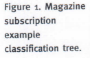
SVMs fit in the context of classification where the attribute whose value is to be predicted (the dependent attribute) has two possible values: 0 or 1. SVM classification is performed by a surface in the space of predictor attributes separating points with dependent attribute = 0 from those with dependent attribute = 1. An optimal separating surface is computed by maximizing the margin of separation (see Figure 2). The margin of separation is the distance between the boundary of the points with dependent attribute – 0 and the boundary of those with dependent attribute = 1. The margin is a measure of “safety” in separating the two sets of points – the larger the better. In the standard SVM formulation, computing the optimal separating surface requires solving a quadratic optimization problem.
The burden of solving the SVM optimization problem grows dramatically with the number of training records. To reduce this burden, a method called “chunking” iteratively updates the separator parameters over chunks of training cases; the size of a chunk is chosen so it fits into main memory. To obtain optimal classification, chunks often need to be revisited, implying multiple passes over the data.
A data compression approach called “squashing” is also applicable to SVM training, where the training records are summarized by a smaller data set emulating the distribution of the original training records. The training records are clustered utilizing the likelihood profile of the data. The SVM is then trained over the clusters, where each cluster is weighted by the number of data points it contains.
Another approach to scaling SVMs involves reformulating the underlying optimization problem, resulting in efficient iterative algorithms. Methods require the solution of a linear system of equations with size m + 1 at each iteration or deal directly with the underlying optimality conditions (Karush-Kuhn-Tucker conditions) to incrementally improve the classification at each iteration; m is the number of predictor attributes.
The SVM predictive function can be decomposed as the linear combination of functions of training data points (called kernels). Projection methods aim to approximate the combination of all training data with a subset of points. Some projection methods use m randomly selected points on which to base the separating surface. Sparse, greedy matrix approximations try to determine the best m points to use.
Clustering
Clustering aims to partition a set of records into several groups such that “similar” records are in the same group according to some similarity function, identifying similar subpopulations in the data. For example, a cluster could be a group of customers with similar purchase histories, interactions, and other factors: for an overview on clustering, see (5, 6).
One scalability technique for clustering algorithms is to incrementally summarize dense regions of the data while scanning a data set. Since a cluster corresponds to a dense region, the records within this region can be summarized collectively through a summarized representation called a “cluster feature” (CF), such as the triple consisting of the number of points in the cluster, the cluster centroid, and the cluster radius. More sophisticated cluster features are also possible.
CFs are efficient for two reasons: they occupy less space than maintaining all objects in a cluster; and if designed properly, they are sufficient for calculating all inter-cluster and intra-cluster measurement for making clustering decisions. Moreover, these calculations can be performed faster than using all objects in clusters. Distances between clusters, radii of clusters, and CFs – and hence other properties – of merged clusters can all be computed quickly from the CFs of individual clusters.
CFs have also been used to scale iterative clustering algorithms, such as the K-Means algorithm and Expectation-Maximization algorithm (5, 6). When scaling iterative clustering algorithms, the algorithm identifies sets of discardable points, sets of compressible points, and a set of main-memory points. A point is discardable if its membership in a cluster can already be ascertained with high confidence; only the CF of all discardable points in a cluster is retained while the actual points are discarded. A point is compressible if it is not discardable but belongs to a tight subcluster consisting of a set of points that always move between clusters simultaneously. The remaining records are designated as main-memory records, as they are neither discardable not compressible. The iterative clustering algorithm then moves only the main-memory points and the CFs of compressible points between clusters until a criterion function is optimized.
Other research on scalable clustering focuses on training databases with large attribute sets. The search methods involve discovering the appropriate subspace of attributes in which the clusters are most likely to exist. These methods help analysts trying to understand the results, as they focus only on the attributes associated with a given cluster.
Association Rules
Association rules (5 – 7) capture the set of significant correlations present in a given data set. Given a set of transactions, where each transaction is a set of items, an association rule is an implication of the form X=> Y, where X and Y are sets of items. This rule has support s if s% of transactions include all the items in both X and Y, and confidence c if c% of transactions containing X also contain Y. For example, the rule “[Carbonated Beverages] and [Crackers] => [Milk]” might hold in a supermarket databases with 5% support and 70% confidence. The goal is to discover all association rules with support and confidence greater than the user-specified minimum support and minimum confidence, respectively. This formulation has been extended in many directions, including the incorporation of taxonomies, quantitative association, and sequential patterns.
Algorithms for mining association rules usually have two distinct phases. First, they find all sets of items with minimum support (in other words, the frequent itemsets). Since the data may consist of millions of transactions, and the algorithm may have to count millions of potentially frequent (candidate) itemsets to identify the frequent ones, this phase can be computationally expensive. Next, rules can be generated directly from the frequent itemsets, without having to fo back to the data. The first step usually consumes most of the time; hence, research on scalability focuses here. Scalability techniques can be partitioned into two groups: those that reduce the number of candidates that need to be counted; and those that make the counting of candidates more efficient.
In the first group, identification of the antimonotonicity property that all subsets of a frequent itemset must also be frequent proved to be a powerful pruning technique that dramatically reduces the number of itemsets that need to be counted. Subsequent research has focused on variations of the original problem. For instance, for data sets and support levels where the frequent itemsets is intractable, since a frequent itemset with n item has 2n frequent subsets. However, the set of maximal frequent itemsets can still be found efficiently by looking ahead; once an itemset to be counted (see the survey in [1]. The key is to maximize the probability that itemsets counted by looking ahead are actually frequent. A good heuristic is to bias candidate generation so the most frequent items appear in the most candidate groups. The intuition behind this heuristic is that items with high frequency are more likely to be part of long frequent itemsets.
In the second group of techniques, nested hash tables can be used to efficiently check which candidate itemsets are contained in a transaction. This is very effective when counting shorter candidate itemsets, less so for longer candidates. Techniques for longer itemsets include database projection, where the set of candidate itemsets is partitioned into groups such that the candidates in each group share a set of common items. Then, before counting each candidate group, the algorithms first discards the transactions that do not include all the common items: for the remaining transactions, it discards the common items (since it knows they are present), as well as items not present in any of the candidates. This reduction in the number and sie of the remaining transactions can yield substantial improvements in the speed of counting.
From Incremental Model Maintenance to Streaming Data
Real-life data is not static, evolving constantly through additions and deletions of records; in some applications, such as network monitoring, data arrives in such high-speed data streams it is practically impossible to store it for offline analysis. A framework we call “block evolution” illustrates these models of evolving data. The input data set to the data mining process is not static, as it is updated with a new block of tuples at regular time intervals, say, every day at midnight (a “block” is a set of tuples added simultaneously to the database.) For large blocks, this model captures the common practice in many data warehouse installations, whereby updates from operational databases are batched together and performed in a block update. For small blocks (in the extreme, a single record), the model captures streaming data.
For evolving data, two classes of problem are of particular interest: data mining model maintenance and change detection. Model maintenance aims to maintain a data mining model undergoing insertion and deletion of blocks of data. Change detection aims to quantify the difference in terms of data characteristics between two blocks of data.
Recent research has focused on mining evolving data. Incremental model maintenance has also received attention, since it is desirable to go from incremental updates to existing data mining models, especially in light of the very large size of data warehouses. Incremental model maintenance algorithms concentrate on computing exactly the same model as if the original model construction algorithm was run on the combined collection of old and new data. One scalability technique widespread in model maintenance algorithms is the localization of changes for inserting new records. For example, for density-based clustering algorithms [6], inserting a new record affects only clusters in the neighborhood of the record; thus efficient algorithms “localize” the change to the model without having to recompute the complete model. Another example involves decision tree construction, whereby the split criteria at the tree might change only within certain confidence intervals under insertion of records, assuming the underlying distribution of training records is static.
When working with high-speed data streams, algorithms have to be able to construct data mining models while looking at the relevant data items only once and in a fixed order (determined by the stream-arrival pattern) with a limited amount of main memory. Data-stream computation has given rise to several recent (theoretical and practical) studies of online and one-pass algorithms with limited memory requirements for data mining and related problems; examples include: computating quantiles and order-statistics; estimating frequency moments and join sizes; clustering and decision tree construction; estimating correlated aggregates and computing one-dimensional, or single-attribute, histograms; and Haar wavelet decompositions. Scalability techniques include: sampling; summary statistics; sketches (small random projections with provable performance guarantees); and online compression of sufficient statistics [2].
Conclusion
Large and growing databases are commonplace in business organizations, governments, and scientific applications. Prior to the invention of scaling techniques, sampling was the primary method for running conventional machine learning, statistical, and other analysis algorithms on these databases. However, this approach also involved having to determine sufficient sample size, as well as the validity of discovered patterns or models (the patterns may be an artifact of the sample). We view sampling as orthogonal and complementary to scaling techniques allow the use of much larger data sets.
The research effort on scaling data mining algorithms to large databases has now given analysts the ability to model and discover valid, interesting patterns over these large data sets. General scaling principles include: use of summary statistics; data compression; pruning the search space; and incremental computation. We described these principles in the practical context of mining algorithms, expecting they would be useful in other areas of computer science as well.
Scalability in data mining is an active area of research, though many challenging questions remain, including the following:
- Can we mine patterns from huge data sets while preserving the privacy of individual records and the anonymity of the individuals who provided the data?;
- What are suitable data mining models for high-speed data streams, and how can we construct them?; and
- In light of the plethora of huge and growing sets of linked data available today, including in the Internet, newsgroups, and new stories, what type of knowledge can we mine from these resources, and can we design scalable algorithms for them?
Source: Communications of the ACM