
Abstract— This paper presents a system called Splash, which integrates statistical modeling and SQL for the purpose of adhoc querying and analysis. Splash supports a novel, simple, and practical abstraction of statistical modeling as an aggregate function, which in turn provides for natural integration with standard SQL queries and a relational DBMS. In addition, we introduce and implement a novel representatives operator to help explain statistical models using a limited number of representative examples.
We present a proof-of-concept implementation of the system, which includes several performance optimizations. An experimental study indicates that our system scales well to large input datasets. Further, to demonstrate the simplicity and usability of the new abstractions, we conducted a case study using Splash to perform a series of exploratory analyses using network log data. Our study indicates that the query-based interface is simpler than a common data mining software package, and for ad-hoc analysis, it often requires less programming effort to use.
I. INTRODUCTION
Data mining is often performed as an iterative, exploratory process involving multiple ad-hoc tasks. Recent work has begun to consider exploratory mining paradigms [22], but most data mining software still supports a rigidly-defined set of tasks (e.g., classification with a fixed training set and class label, or anomaly detection based on a fixed set of models). In contrast, relational databases have been extremely successful in providing simple languages that allow users to specify a variety of ad-hoc queries. Further, many years of research have resulted in database systems that easily scale to large data.
The goal of this work is to develop a system that combines the power of data mining (particularly statistical modeling) with the ad-hoc query power and scale of SQL and relational databases. One motivating application for such a system, which we find particularly interesting, is the flexible ad-hoc analysis and exploration of logs for the purpose of anomaly and misuse detection. \
A. Motivating Example: Log Analysis
Maintaining audit logs is a fundamental component of a comprehensive security [5] and privacy [19] infrastructure. Logging is complementary to access control and other security mechanisms, and it is particularly useful for recording and detecting inappropriate access and misuse by insiders.
To illustrate the importance of audit logs in database management, consider a large healthcare organization, which must take precautions to safeguard sensitive information, including patients’ medical records. The organization has deployed a comprehensive security infrastructure, but due to the evolving nature of care (e.g., residents and nurses who change departments frequently), it is often impossible to specify comprehensive access control policies. In fact, overly-restrictive policies interfere with patient care. Instead, rather than preventing inappropriate access, it is often necessary to take steps to detect such access after the fact by keeping a record of what information has been accessed, and by whom [16]. As a recent example, Kaiser Permanente recently fired fifteen employees for inappropriately viewing the medical records of Nadya Suleman, the highly-publicized mother of octuplets [21].
Legislation and regulatory oversight have required organizations in a variety of domains to track their use of sensitive data [1], [15], [14], but few tools have been developed to allow auditors to systematically and proactively analyze the resulting logs. In healthcare compliance, it is common to focus auditing efforts on a few VIPs (high-profile patients) [16], but this is not a comprehensive solution.
Anomaly detection is one common tool for behavior-based log analysis and intrusion detection, which has been researched extensively for operating systems [27], networks [43], and more recently for database systems [33]. At a high level, the idea is to learn a model of “normal” behavior, and then detect deviations from normal as potential misuse. Unfortunately, even in domains such as operating systems and networks, where anomaly detection has been studied extensively, it is known to have significant disadvantages, including the bothersome problem of false positives [43], and a notable lack of flexibility. For example, a security administrator must decide (a priori) the granularity at which to model behavior (e.g., user, role, process, source IP, etc.), and the output of the system is limited to simple boolean decisions (raise a warning or not).
Thus, inspired in part by the log analysis problem, we set out to build a system that marries statistical models (following the past successes of anomaly detection) with the ad-hoc flexibility and simplicity of high-level query languages.
B. System Requirements
We identified three high-level requirements for Splash:
• Scalability: Our system should be able to scale gracefully to large input datasets, particular those that are signifi- cantly larger than main memory.
• High-Level Query Language: The system should support a simple high-level query language that allows easy specification of ad-hoc queries and analyses with minimal programming effort.
• Natural Abstraction for Statistical Models: The data model and query language should provide a simple and natural abstraction for ad-hoc creation and direct manipulation of models.
While statistical software (e.g., Matlab [7], R [9], Stata [12], SAS [11]) and data mining packages (e.g., Weka [13]) provide a great deal of statistical modeling functionality, to the best of our knowledge all assume that the data to be analyzed is small enough to fit in main memory. Recent work has proposed techniques that allow R to scale to larger datasets [50]. However, none of these software packages provides a high-level query language, which makes ad-hoc exploratory analysis somewhat more difficult than in a typical SQL database because the user must write a custom program for each new analysis. Further, these tools do not typically support automatic optimization and operator re-ordering as is found in relational databases.
For all of these reasons, several systems have proposed incorporating support for statistical and data mining models into relational databases and SQL. Two specific abstractions have been proposed. However, we find that neither provides a natural abstraction for ad-hoc model creation and manipulation, specifically in the log analysis domain.
MauveDB [24] provides a novel abstraction called a modelbased view. The idea of this abstraction is to expose to the user data interpolated from the model, as if this data were part of an ordinary database view. While this abstraction is natural for data interpolation (e.g., in the sensor domain), it suffers two main shortcomings when it comes to ad-hoc analysis: (1) Each model must be declared using syntax similar to SQL’s CREATE VIEW, which leads to a tedious process if an analyst wants to create many models (e.g., one per system user in the log analysis domain), and (2) Aside from the interpolated views, models are completely hidden from the user. This makes it difficult, for example, to use a model-based view for the purpose of detecting anomalies (records that deviate significantly from a given model), or for comparing models.
Microsoft SQL Server’s DMX [2] and OleDB for DM [41] expose classification and regression models through an abstraction known as a prediction-join. This abstraction provides a natural way of assigning class labels to data, but it does not allow a user to compare a record to a model, or to compare two models (e.g., for the purpose of detecting anomalies). Also, like MauveDB, the user must specify each model separately using extended SQL DDL, which can be cumbersome.
C. Summary of Contributions
We have designed and built a system called Splash. Splash supports the novel abstraction of statistical models as SQL aggregates, which allows for easy, ad-hoc, set-oriented specification and manipulation of models using standard SQL (Section II). In addition, we propose a novel representatives operator, and algorithms, which help to explain a model using a small set of examples (Section III). Section IV describes the details of out prototype implementation, including performance optimizations.
An extensive experimental study (Section V) evaluates three main aspects of Splash: First, we evaluated performance and scale. Second, we compared algorithms for implementing the representatives operator. Finally, we conducted a case study using network attack logs to evaluate our newly-proposed abstractions; we found that ad-hoc analyses are often more easily expressed using the query language of Splash than using a common open-source data mining package.
II. DATA MODEL & QUERY LANGUAGE
The data model and query language supported by Splash are based on the relational model and SQL, but incorporate support for statistical models as a new data type (like an integer or string). Ad-hoc model construction is naturally viewed in terms of a new aggregate function (similar to SUM or AVG).
A. Basics
Splash allows ad-hoc creation and querying of profiles, statistical models describing the contents of any set of records. In the log analysis example, where each record represents a system interaction or request, a profile can be used, for example, to describe the typical behavior of a user, or requests issued from a particular IP address.
Of course, before constructing a profile, it is common to extract appropriate features from the input records. This is done via the feature extractor function.
Definition 1 (Feature Extractor): The feature extractor, denoted features(), is a user-replaceable function, which takes as input a database record, and produces a feature vector of the form (X1, …, Xn)1.
Using a set of extracted feature vectors as input, a profile aggregation operator constructs a profile, which is a probabilistic model describing the input feature vectors.
Definition 2 (Profile): A profile is an estimated joint probability density function (pdf) over the space of features.2 We will denote a profile constructed over features X1, …, Xn as fX1,…,Xn (x1, …, xn).
Definition 3 (Profile Aggregation Operator): Let D be a set of records with extracted features X1, …, Xn. profile(D) is an aggregate function that produces a profile object.
The profile aggregation operator is also easily extended to first partition D based on some attribute P, and then construct one profile per unique value p of P. (This is similar to a SQL GROUP BY query.)
These basic building blocks are nicely integrated with standard SQL, and this is best illustrated with an example. Suppose that we have a relation AuditRecords(RID, USER ID, A1,…, Am), where RID is a key, and USER ID identifies the system user associated with each audit record. In (slightly extended) SQL syntax, feature extraction is expressed follows: CREATE VIEW FeatureVectors(RID, USER_ID, featureVector) AS SELECT RID, USER_ID, features(A1,…,Am) FROM AuditRecords
Ah-hoc profile aggregation is easily expressed using standard SQL aggregation and GROUP BY syntax. For example, we can create one profile per user: SELECT profile(featureVector), USER_ID FROM FeatureVectors GROUP BY USER_ID
B. Sample Profile Aggregation Operator
The idea of a profile as a probability density function is very general, and there are countless ways to estimate fbX1,…,Xn (x1, …, xn) from D. Our main objective is to provide a clean abstraction for integrating SQL and probabilistic models, not to develop new machine learning techniques. This section briefly describes the profile operation that we have implemented in our prototype system; however, this is not fundamental to the data model, and can easily be replaced.
For the purposes of our prototype, we constructed a profile aggregation operator using the simplifying assumption that features X1, …, Xn are conditionally independent, given profile attribute P. 3 That is, assume that fX1,…,Xn (x1, …, xn) = Qn i=1 fXi (xi), and estimate each fbXi (x) separately.
When Xi is discrete-valued, fXi is a probability mass function, and it is easy to estimate using counts: fbXi (x) = |{d∈D:d.Xi=x}| |D| . (To avoid the case where some counts are zero, a simple adjustment adds one to the numerator and denominator.)
When Xi is continuous, we estimate the probability density function using a Gaussian kernel density estimator. If h is a smoothing parameter and K(x) = √ 1 2π e − 1 2 x 2 , then we define fbXi (x) = 1 |D|·h P d∈D K( x−d.Xi h ).
C. Query Language
In providing extensions to SQL, our goal was to integrate standard ad-hoc relational queries with direct manipulation of statistical models. In Splash, profiles are exposed and manipulated primarily through two new primitive functions:
Similarity between a feature vector and a profile: The similarity between a feature vector and a profile is denoted sim(x1, …, ni, p), and is a real number in the range [0, 1]. Suppose that profile p is defined by estimated distribution fbX1,…,Xn . One way of defining the similarity is to let sim(x1, …, xn, p) = fX1,…,Xn (x1, …, xn). When one or more of the features Xi is continuous, a simple adjustment integrates fXi over an interval (±δ) surrounding xi .
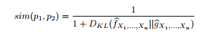
Similarity between two profiles: The similarity between two profiles is denoted sim(p1, p2), and is also a real number in [0, 1].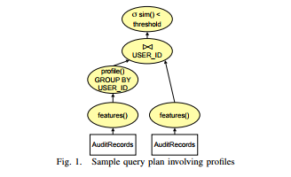
Suppose that profiles p1 and p2 are defined, respectively, by estimated distributions fbX1,…,Xn and gbX1,…,Xn . The KL-divergence is one common information-theoretic way of measuring the difference between two distributions:4
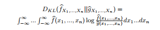
We can use this to construct a similarity function:
Using the primitive similarity functions as building blocks, it is possible to compactly express a variety of useful composite queries, combining standard SQL data manipulations with queries on profiles. This list is not intended to be exhaustive; for more examples, see the case study in Section V-B.
Detecting anomalous records: Of course, we can easily express the query requesting anomalous records, defined as any record such that the similarity between the record and its associated profile is less than a given threshold. This is expressed as follows; a sample query plan is shown in Figure 1.
SELECT F.RID FROM FeatureVectors F,
(SELECT profile(featureVector), USER_ID FROM FeatureVectors
GROUP BY USER_ID) AS Profiles(P, USER_ID) WHERE F.USER_ID = Profiles.USER_ID AND sim(F.featureVector, P) < threshold
Instead of profiling behavior at the level of individual users, this query could easily be modified to construct profiles in a different way. For example, if we had an attribute ROLE ID, we could easily use that instead.
Ranking anomalous records: It is also easy to request a ranked list of potentially anomalous records. This can be done by removing the threshold, and adding ORDER BY sim(featureVector, P) ASC to the previous query. In Figure 1, the selection operator (σsim()<threshold) would be replaced with a sort operator.
Detecting changes over time: Continuing with the log analysis example, we can also construct a query to discover the users whose behavior has changed significantly since the previous month. (For this example, suppose that the view FeatureVectors also contains an attribute MONTH.)
SELECT Profile1.USER_ID
FROM (SELECT profile(featureVector), USER_ID
FROM FeatureVectors
WHERE MONTH = ’May’
GROUP BY USER_ID) AS Profile1(P, USER_ID),
(SELECT profile(), USER_ID
FROM FeatureVectors
WHERE MONTH = ’June’
GROUP BY USER_ID) AS Profile2(P, USER_ID) WHERE Profile1.USER_ID = Profile2.USER_ID AND sim(Profile1.P, Profile2.P) < threshold
III. PROFILE EXPLANATION AND FINDING REPRESENTATIVES
Aggregation provides a natural way of creating profiles, and the sim() functions provide for basic interaction with profile objects. However, the user may want to further understand the meaning of certain profiles. For example, in log analysis, a system administrator may have detected an abnormal profile, which he would like to understand better.
As one means of explaining a profile, we propose an operator that, given a profile p and dataset D, selects a small subset of D to represent the profile distribution. (To keep the operator as general as possible, we do not require that D be a sample from the same distribution as p.) This results in the following optimization algorithm. While related problems have been considered in the literature (see Section VI), to the best of our knowledge, this problem has not been addressed.
Definition 4 (Representative Set): Given a profile p, a set of feature vectors D, and user-defined parameter k, the optimal representative set, denoted rep(p, D, k), is the set D’ ⊆ D such that |D | ≤ k and sim(p, prof ile(D0′)) is maximized.
In the above, profile(D’) represents the pdf derived from the points in D’ after applying kernel density estimation, and sim(p1, p2) is the same similarity function described earlier.
Due to the combinatorial nature of the problem, we have developed several heuristics for selecting representative sets. Empirically (Section V-D), we observe that one of the algorithms (GREEDY-R) works extremely well in practice.
A. Algorithms
When describing the algorithms, we regard each of the m feature vectors in D as a point in an n-dimensional space.
Sampling Algorithm (RAND-R): The simplest (naive) approach is to choose a simple random sample from D. While sampling is widely used in statistics, there are two clear problems to using this approach here. First, while profile(D’) will converge to p (for large k) if D is drawn from the distribution p, RAND-R is only effective in this case. When profile(D) 6= p, profile(D’) converges to profile(D) rather than p. Second, even when RAND-R is guaranteed to converge for large k, we would ideally like to choose a subset that is as small as possible.
Histogram-Based Sampling (HIST-R): To overcome the shortcomings of RAND-R, one approach is to actively allocate the positions of representative points. This can be done by partitioning the space into subregions, and allocating representatives to each subregion based on the region’s probability mass in p5.
To partition the space, we leverage the well-known multidimensional histogram partition rule MHIST [44] and the partition constraint V-optimal [32]. The partition algorithm is recursive; it begins by dividing the whole space into two regions, and then recursively partitions each of the resulting regions until a stopping criterion is met. Each iteration proceeds as follows. (Suppose that we are working on subregion R, which contains m∗ points from D, and based on probability mass, we need to select k ∗ representative points from this subregion).
1) Select a dimension to divide. (The dimension with maximum variance in p is selected, following the MHIST heuristic.)
2) Choose the point at which to divide the selected dimension. (We choose the point according to the V-optimal criterion.)
3) Divide the m∗ points between the resulting subregions R1 and R2, and set k ∗ 1 and k ∗ 2 (the number of representatives that need to be chosen from R1 and R2) according to the probability mass of p in R1 and R2.
The partitioning process continues recursively until m∗ = k ∗ or k ∗ = 1, at which point we randomly select k ∗ points from those in D that fall in the subregion (R). There are O(k) iterations. In each iteration, Step 1 takes O(n) time, Step 2 takes O(c) time where c is the number of distinct values in the chosen dimension, Step 3 takes O(m) time. Therefore the running time for the algorithm is O((c + n + m)k).
While this approach eliminates some of the problems of RAND-R in that it can be used when D and p do not have the same distribution, it is also highly dependent on the partitioning algorithm. In high-dimensional space, histograms are known to deteriorate in quality. (This is confirmed by our experiments.) Thus, we propose a third and final algorithm.
Greedy Algorithm (GREEDY-R): To overcome the limitations of HIST-R, we propose a third algorithm called GREEDY-R, which incrementally selects the next most representative point. Remember that a kernel density estimation based on k points just sums up the k kernels, using a weight w = 1 k for each. The process of the greedy algorithm is to incrementally add representative points into D’ ; for each new point d, we incrementally maintain a partial profile p‘ by adding the kernel for d using weight w = 1 k . (For |D0 | < k, p’ is not a true probability distribution.) The difference between p and p’ at d is denoted δ(p, d) = p − p’ .
The greedy algorithm works as follows: At each step, we choose the point d from D − D’ that maximizes δ(p, d). This process repeats until all k representative points are chosen. The intuition behind the heuristic is that at each step we always look for points that minimize the gap between the profile p and the sum of the kernels p’. We demonstrate the effectiveness of the algorithm in Section V.
The greedy heuristic takes k steps. At each step it takes O(mn) time to pick the best point as next representative point and to update the partial distribution after a point is picked. Therefore the running time for the greedy heuristic is O(kmn).
IV. IMPLEMENTATION
We have built a prototype of Splash using extensions to PostgreSQL [8]. In addition, we have implemented several performance optimizations based on materialization and compression of profiles. A. Overview
The prototype was built using extensions to PostgreSQL [8], an open-source DBMS that supports user-defined types, operators, functions, and aggregates. It is noteworthy that all of the functionality can be implemented without costly modifications to the database engine. We defined new types to represent profiles and feature vectors, and functions to support operations on profiles and feature vectors. All of the extensions are implemented using C. The following is a list of the new types, functions, aggregates, and operators:
• Feature is a new type representing a feature vector. (The dimensionality of a Feature instance is the length of the vector.) In the current implementation, we support feature entries of types integer, varchar, varbit, and real.
• Profile is another new type. In our prototype, we implement a profile using a collection of n hash tables, where n is the total number of different features. The ith hash table contains all distinct values of feature Xi (the keys) and an integer count for each. Thus, the space required to store a Profile instance is O(cn), where c is the average number of different values per feature. We use this representation for both discrete and continuous features; the differences in probability estimation (i.e., count-based or kernel density estimation) are encapsulated by the two similarity functions.
• profile(Feature) is a new aggregate function, which produces a Profile instance, given a set of Feature instances. In PostgreSQL, user-defined aggregates are expressed in terms of state values and state transition functions. For this reason, we have defined the transition function profile(Profile, Feature) to enable adding one Feature instance to an existing Profile. Assuming that there are m Feature vectors, each with dimensionality n, in this implementation, the time complexity of adding one Feature value to a Profile is O(n), and the time complexity of building a Profile from m Feature vectors is O(mn).
Of course, this approach assumes an implementation of Profile that is incrementally updatable. This is clearly a desirable characteristic of the profile model. For other profile models, we might need to maintain additional state. In addition, the query optimizer treats queries involving profile aggregation just as it would treat any other aggregate query. For the most part, this works reasonably well, but there are some unexpected problems, as we discuss in more detail in Section V.
• sim(Feature, Profile) is a function that evaluates the similarity between a Feature instance (x1, …, xn) and a Profile instance p, as described in Section II. For discrete feature Xi , we can compute fXi|P =p(xi) in O(1) time from the internal profile representation. For continuous feature Xi , we can compute R xi+δ xi−δ fXi|P =p(x), in time O(c), where c is the number of distinct values for Xi . Therefore, when all features are discrete, we can compute this function in O(n) time; otherwise it takes O(cn).
• sim(Profile, Profile) is a function that evaluates the similarity between two Profile instances using the KL-divergence as described in Section II. We observe that, due to the conditional independence assumption, it is possible to compute the KL-divergence for each feature independently. The observation is captured by following theorem:
Theorem 1:
![]()
Proof:
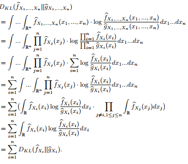
Thus, this function is straightforward for discrete features, and can be computed in O(cn) time, where n is the dimensionality of the feature vector, and c is the number of distinct values per feature. When one or more of the features Xi is continuous, we handle that by discretizing the range of Xi into r discrete ranges, and then estimate the probability density within each range using the stored counts and kernel density estimator. In this case, the time complexity is O(rcn).
B. Materialization
Aggregate materialization is commonly used to improve performance in OLAP-style data analysis. In much the same way, it may be useful to materialize profiles to improve the performance of certain workloads in Splash. For example, each of the sample queries in Section II-C required computing one profile per USER ID. However, it is also likely that the user would like to view profiles at different levels of granularity (e.g., one profile per RBAC ROLE ID). Just like OLAP, it is convenient to think of these different granularities as forming a partial order [28].
Of course, even for conventional aggregates (which are typically integers or reals), fully-materializing an entire data cube is space-consuming, and because profile objects are larger than integers or reals, dealing with space consumption is an even bigger issue here. To select the best set of profiles, given limited space, we implemented the heuristic proposed by Harinarayan et al. [29] in a separate Planner module.
To answer queries involving a particular profile, when the profile cube has been partially materialized, we first check to see whether the desired profile has been materialized. If it has, then it can be used directly. Otherwise, ideally, we would like to compute the desired profile from a set of (materialized) constituent profiles at a finer level of granularity. (For example, if a query requests profiles grouping-by ROLE ID, we would like to be able to compute these profiles directly from the set of profiles grouping-by USER ID, rather than using the original data.) Like standard aggregate data cubes, this is captured by the idea of distributive and algebraic aggregates; an aggregate function is algebraic if it can be computed from intermediate statistics at finer levels of granularity [28]. Our internal profile representation is algebraic; the internal counter representation can be computed from profiles at finer granularities without accessing the underlying data. More generally, recent work showed that Naive Bayes classifiers and kernel density estimators are algebraic aggregates [22].
C. Profile Compression
Materializing profiles can still be space-consuming, particularly if there are many distinct values for certain features. Thus, it is beneficial to consider compressing materialized profiles. One approach is to replace each of the n counter vectors with a histogram. We apply V-Optimal histogram [32] to each dimension to compress the vector of counts representation. The effect of compression is demonstrated in Section V-C.
Practically-speaking, compression is incorporated into our prototype via a function compress(Profile). We envision applying compression to archived profiles constructed over historical data (e.g., from past years or months) that is no longer being updated.
V. EXPERIMENTAL EVALUATION
We conducted an extensive experimental study using the Splash system, designed to measure the following:
• Performance and Scale: One of our guiding principles was to develop a system that scales to large datasets. We measured the performance and scalability of Splash, including the effects of materialization and compression.
• Query Language and Profile Abstraction: To provide a greater understanding of the flexibility provided by Splash, we performed a case study comparison. Using a wellknown dataset from the network intrusion domain, and an interesting set of ad-hoc exploratory analysis tasks, we compared the process of expressing these tasks in Splash with the process of expressing these tasks in an open-source data mining package called Weka [13].
• Generating Representatives: Finally, we evaluated and compared the algorithms described in Section III for generating representatives.
We ran our experiments on a machine with Pentium dualcore 2GHz CPU and 2GB memory. We used the Ubuntu 8.04 operating system and PostgreSQL 8.3. The size of sharedmemory for PostgreSQL was set to 512MB.
A. Performance & Scale
Our first set of experiments were designed to measure the performance and scalability of Splash when used for large input datasets.
1) Data Generator: For these experiments, we used a simple synthetic data generator, which produces data with the following schema:
SynData(yy, mm ,dd, featureVector)
yy, mm, and dd are hierarchical dimension attributes representing the date. featureVector is a 10-dimensional feature vector. We generated the values of the features using Gaussian distributions; however, since the synthetic data is used only for testing performance and scale, the distribution is of relatively little importance. Each resulting record is approx. 150 bytes.
For each distinct day, we generated 1000 records. (The average profile size per day is 40KB.) In the experiments, we vary the number of days (months, and years), in order to vary the size of the dataset. The maximum data size is 30 years (roughly 100 million records), which consume 15GB of total space.
2) Scale-Up: To evaluate how Splash scales to large input datasets, we varied the input data size from 100 days ( 150MB of data) to 10,000 days ( 15GB of data), and we issued the following profile construction query:
SELECT profile(featureVector)
FROM SynData
GROUP BY yy,mm,dd
The size of the profiles resulting from this query ranges from 40MB to 4GB. For the sake of comparison, we also tested the built-in aggregate sum() on the same input. The results of this experiment are shown in Figure 2(a-c).
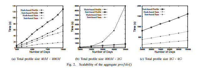
In Figure 2(a), notice that when the data size is small, the profile() aggregate works pretty well (using approximately 4 times as much time as sum()). However, as the data size grows, the running time for profile() suffers significantly. After analyzing the query plan, we discovered that the PostgreSQL query optimizer always selected a hash-based aggregation operation instead of a sort-based plan. However, the total size of the resulting profiles grows much larger than traditional aggregates, and when the hash table containing these profiles can no longer fit in the shared buffer, the query begins to thrash.6
On the other hand, if we force the system to use a sort-based plan to evaluate profile() aggregates, we do not encounter this problem. To force PostgreSQL to use a sort-based plan, we explicitly perform the sort as part of the query:
SELECT profile(featureVector)
FROM (SELECT * FROM SynData ORDER BY yy,mm,dd)
GROUP BY yy,mm,dd
In Figure 2(a), when the data is small, the sorting-based prof ile() is a bit slower than the hash-based profile() due to the overhead of sorting. However, as the data size grows, and the hash-based profile() begins to thrash (Figure 2(b)), the sort-based operation is not significantly affected. As we keep growing the total size of profiles to 4GB (Figure 2(c)), which is larger than 512MB shared-buffer and 2GB memory, the sort-based profile() still scales well.
3) Effects of Materialization: To demonstrate the effectiveness of materialization, we vary the size of data from 1 year (500M data) to 10 years (5GB data). Suppose that we have constructed (using the synthetic data) a partial materialization including one profile per day, as defined by the following view: CREATE MATERIALIZED VIEW ByDay AS
SELECT yy, mm, dd, profile(featureVector)
FROM SynData
GROUP BY yy, mm, dd
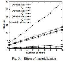
The size of the materialized view varies from 133MB (for 1 year) to 1.33GB (for 10 years). Now, consider the following three queries, each of which can be evaluated either using the materialized table (ByDay) or using the base data (SynData).
1) SELECT sim(profile,featureVector) FROM SynData F, (SELECT yy,mm,dd, Profile(featureVector) FROM SynData
GROUP BY yy,mm,dd) AS P(yy,mm,dd,profile)
WHERE P.yy=F.yy AND P.mm=F.mm AND P.dd=F.dd
2) SELECT sim(profile,featureVector) FROM SynData F,
(SELECT yy,mm, Profile(featureVector)
FROM SynData
GROUP BY yy,mm) AS P(yy,mm,profile)
WHERE P.yy=F.yy AND P.mm=F.mm
3) SELECT sim(profile,featureVector)
FROM SynData F, (SELECT yy Profile(featureVector)
FROM SynData GROUP BY yy) AS P(yy,profile)
WHERE P.yy=F.yy
Figure 3 shows the performance of each query using the materialized table (“Mat”) and using the base data. The running time drops substantially when the materialized table is used. For the two queries that use profiles grouping by month and by year, although no materialized table can be used directly (i.e., ByMonth or ByYear), calculating these profiles from the materialized ByDay is still more efficient than building them from scratch.
B. Application Case Study
Our next set of experiments evaluates the flexibility afforded by a high-level query language incorporating profiles. For this purpose, we conducted a case study for network attack logs. The idea is to consider a security administrator and the ad-hoc exploratory tasks he or she would conduct to understand the logged information. We chose this particular domain because anomaly-based intrusion detection has been well-studied for networks, and there exist established benchmark data sets.
Existing data mining and statistical software packages (e.g., Weka [13], Matlab [7], and R [9]) do not provide flexible high-level query languages. This means that if a user wants to make advanced use of statistical or mining primitives (e.g., embedding in a larger analysis), then she must write a custom procedural program each time. Further, query optimization strategies cannot be automatically incorporated into these programs, so the user also needs to worry about optimization each time she writes such a script.
For our case study, we developed a sequence of exploratory tasks, and we compared the programming effort required to express these tasks using Splash and using Weka [13]. We observed that it is relatively easy to express conventional tasks (e.g., simple classification) in both systems, primarily because Weka provides a custom API for these tasks. However, when the analysis task involves additional data processing, or compound tasks, it is necessary to embed calls to the Weka API in a larger (custom-coded) program, which is inconvenient and time-consuming for ad-hoc analysis. In contrast, compound tasks can usually be expressed quite easily in Splash.
1) Network Attack Data: For the case study, we used the KDD Cup 1999 dataset[6], which has been heavily studied, and is considered a benchmark for data mining techniques and intrusion detection. The data set consists of a set of Internet connection records (a connection is a sequence of TCP packets), each with 41 pre-extracted features (including, for example, the protocol type of the connection, network service type of the destination, and number of data bytes transferred from source to destination).
The connections are divided into five main classes: normal connections (normal), probe attacks (probe), denial-ofservice attacks (dos), user-to-root attacks (u2r), and remoteto-local attacks (r2l). In addition, the four main attack classes can be further decomposed into sub-classes. For example, the dos attack is decomposed into sub-classes that include dos.apache2, dos.mailbomb, and dos.updstorm. The data set consists of 494,021 training records, and 311,029 testing records. We store these data sets (including extracted features) in two tables, where id uniquely identifies each record, featureVector stores the 41 features associated with the connection, class stores the main class label associated with the connection, and subClass stores the sub-class:
TrainingData(id, featureVector, class, subClass) TestingData(id, featureVector, class, subClass)
The KDD Cup contest posed a classification task: Using the training data, construct a model that accurately predicts the attack category (among the 5 main classes) for each of the testing connections. Classification results were evaluated by taking the average error across all classification decisions (on the testing set), so a lower score implies better results. The best reported score in the contest was 0.2331, and results within the range [0.2331, 0.2684] were considered good [10].
2) Case Study Tasks and Results: We performed a series of exploratory tasks (including, but not limited to, simple classification) to help understand the information contained in these logs. For each task, we compared the process of performing the task using Splash with the process of performing the task in Weka [13].
For this comparison, we found a meaningful quantitative measure elusive. When we began the study, we started by comparing the number of lines of code necessary to perform each task in Splash vs. Weka. However, we found that this did not fully convey the distinctions between the two systems. (As one example, some of the tasks could be accomplished in Weka by modifying the engine with a small amount of code, or by writing a larger amount of application code, and it was not clear how to quantify the difference between these two solutions.) Thus, we deliberately chose to provide a qualitative comparison, rather than quantitative measurements.
1. Classification
Task: Classification is a common data mining technique that can be used in network intrusion detection when training data is available describing both normal behavior and attacks [43].
Splash: For simplicity, suppose that we begin by constructing one profile for each of the 5 main class labels:
CREATE VIEW Profiles(class, profile)
AS SELECT class, profile(featureVector)
FROM TrainingData
GROUP BY class
Classification of the testing records is performed by comparing each record with all of the profiles to find the profile with maximum similarity. (For the sample profile construction and similarity functions described in Sections II-B and II-C, the following implicitly trains a Naive Bayes classifier, and uses it to classify the testing records.)
CREATE VIEW MaxSim(id, maxsim) AS
SELECT T.id, max(sim(P.profile, T.featureVector))
FROM TestingData T, Profiles P
GROUP BY T.id
SELECT T.id, P.class
FROM TestingData T, Profiles P, MaxSim M
WHERE T.id = M.id
AND sim(P.profile, T.featureVector) = M.maxsim
We observe that this simple classifier produces a score of 0.258 for the KDD Cup Dataset, which is considered good [10]. While our goal is not to test the profiling algorithm, this is a reasonable model to use when evaluating the query processing and exploratory analysis tool.
Weka: Classification is one of the standard data mining tasks for which Weka provides an explicit API. It is useful to note that training and testing a classifier (e.g., a Naive Bayes model) uses around ten lines of code, which is comparable to the size of the query required by Splash.
2. Anomaly Detection
Task: In contrast to classification, anomaly detection is practical when the only available training data describes normal behavior, rather than malicious or attack behavior. Intuitively, the goal is to construct a model describing normal behavior, and then mark those records that are dissimilar to the model as potential attacks [43].
Splash: We can express anomaly detection in Splash as follows, where thres1 is a parameter provided by the security administrator:
SELECT T.fid
FROM TestingData T, Profiles P
WHERE P.class = ’normal’
AND sim(P.profile, T.featureVector) < thres1
Weka: Weka does not provide an explicit API for anomaly detection, which leaves the user with two options: (1) She can modify the Weka engine (altering the API) in order to add such functionality. (In doing this, she can re-use some of the existing engine-level classification code.) (2) She can write a custom application from scratch to implement anomaly detection.
3. Anomaly Detection Leveraging Attack Data
Task: We observed that classification and anomaly detection each have strengths and weaknesses. In particular, classification cannot identify unknown attacks that do not appear in the training data. However, anomaly detection cannot leverage training data for known attacks [25]. A logical solution exploits both tools: An audit record is considered part of an attack if it is classified as an attack by a classifier, or it is marked as anomalous by an anomaly detector. (Related ideas have been considered in [38], [46], [49].)
Splash: This task combines anomaly detection and classification, and is expressed using the following simple query:
SELECT T.id
FROM TestingData T, Profiles P, MaxSim M
WHERE P.class = ’normal’
AND (sim(P.profile,T.featureVector) < thres1
OR sim(P.profile,T.featureVector) != maxsim)
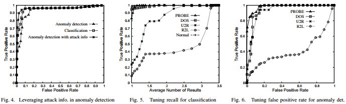
The effects of integrating anomaly detection and classification are shown in Figure 4. Interestingly, this approach outperforms both anomaly detection and classification.
Weka: While Splash provides a convenient set of declarative query operators, in Weka we need to write custom application code encapsulating the basic data mining operations. In this case, the custom application consists of four steps (provided that we have already written a new anomaly-detection module for Weka): (1) Train the classifier; (2) Classify the testing data, and filter those records with class labels other than “normal”; (3) Train the anomaly detector; (4) Identify the anomalies in the remaining testing data. This process consists of two training and two testing phases, which are redundant compared to the Splash query, which constructs a single set of profiles. This redundancy is rooted in the rigid API design of Weka, which does not capture the underlying relationship between statistical anomaly detection and statistical classification. Further, it is the security administrator’s responsibility to take care of interleaving the four phases to make the code efficient.
4. Classification Using a Class Taxonomy
Task: We also observed that the KDD cup data actually includes class labels that are expressed at multiple levels of granularity. While each of the main categories (i.e., dos, etc.) is present in the training data, the testing data contains some new sub-categories that are not present in the training data. Thus, we considered the classification problem of assigning the best class label (at any granularity) to each testing record.
Splash: Splash is particularly well-suited to handle this task. The following constructs a view which contains profiles for all class and sub-classes in the training data:
CREATE VIEW Profiles(class, profile) AS
SELECT class, profile(featurevector)
FROM TrainingData
GROUP By class
UNION
SELECT subClass, profile(featurevector)
FROM TrainingData
GROUP BY subClass
Using this view, the same query as in the classification task can be used to classify each testing record to the most appropriate class (at any level of granularity). In order to compare this to the original result, we mapped the results back to the 5 main classes. Our main goal, of course, is to demonstrate that it is simple to express even complex tasks using Splash. On the other hand, it is interesting to point out that this approach attains a score of 0.228, which is better than any result reported as part of the KDD Cup contest!
Weka: We see two ways of approaching this task using Weka. The first option would extend one of Weka’s classifiers (e.g., Naive Bayes) to make the classifier aware of the hierarchical class labels present in the training data. This requires modifications to the Weka engine and API.
The second option is done entirely at the application level. Notice that the hierarchical relationships between class labels can be handled without modifying the classifier by producing additional training data. For example, if there exists a training record with label attack.dos.apache2, we can generate three training records with labels attack, dos, and apache2. However, this approach unnecessarily expands the size of the training data by a factor of three.
5. Tuning Classification Recall
Task: While classification and anomaly detection tools are powerful, they do not provide the built-in ability to tune the results according to a security administrator’s specification. For example, in the KDD Cup contest, even the winning solution observed very low true positive rates for detecting u2r and r2l attacks (13.2% and 8.4%, respectively). Thus, when conducting an exploratory analysis, the security administrator might consider examining more than one class label per request, as a way of boosting the number of true positives.
Splash: Using Splash, the classification recall can be easily adjusted, simply by modifying thres2 in the following query:
SELECT T.id, P.class
FROM TestingData T, Profiles P, Maxsim M
WHERE T.id = M.id
AND sim(P.profile,T.featureVector) >=M.maxsim-thres2
The effects of tuning thres2 are shown in Figure 5. Notice that by returning an average of 1.4 class labels per testing record, the security administrator can achieve 79.0% and 37.4% recall for the u2r and r2l attacks, which are 3.3 and 4.2 times better, respectively, than the recall rate when returning just one class label per test record.
Weka: The problem of tuning classification recall should be easy to handle in Weka. However, the Weka API is not designed to accept the parameter thresh2, or to return multiple class labels. Thus, to evaluate this task would require some redesign and modifications to the Weka software package.
6. Tuning False Positives for Anomaly Detection
Task: Finally, high false positive rates are a major concern when adopting anomaly detection techniques [43], and the security administrator may want to compromise some true positives for a lower false positive rate. In either case, the ability to tune the result set is critical for exploratory analysis.
Splash: False positives are easily tuned using parameter thres1 in the above anomaly detection query. Figure 6 shows the tradeoff between true positives and false positives. Of course, finding an appropriate thres1 is important in anomaly detection. Given a set of training data, and the maximum allowable false positive rate r, we can estimate the parameter thres1 from the training data. In the following, let n = r · |T rainingData|.
SELECT sim(P.profile,T.featureVector) as thres1
FROM TrainingData T, Profiles P
WHERE T.class = ’normal’
AND P.class = ’normal’
ORDER BY sim(P.profile,T.featureVector)
LIMIT 1 OFFSET n
This query orders the training records based on their similarity to the profile of normal behavior, finds the nth most similar training record, and uses its similarity to the normal profile to set the threshold.
Weka: Weka does not currently support anomaly detection, but if we were to add this functionality, we would need to incorporate thresh1 as a parameter in the API in order to support this task.
C. Effects of Compression
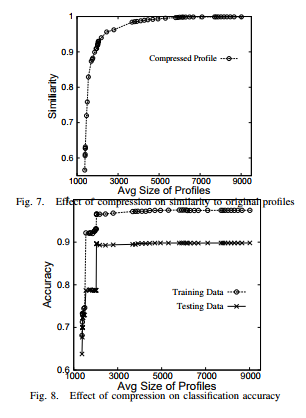
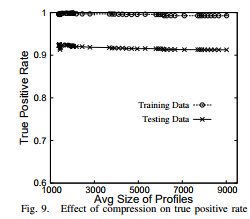
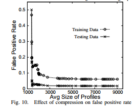
While compression based on histograms, as described in Section IV-C, is effective in reducing the size of profile objects, it also removes some detail from the profiles. To measure the effects of compression, we performed several experiments using the KDD Cup data. In particular, we used four metrics to evaluate the loss of content resulting from histogram-based compression: (1) Similarity between the compressed profile and the original profile (Figure 7), (2) Accuracy of a classifier constructed using the compressed profiles (Figure 8), (3) True positive rate for anomaly detection (Figure 9), and (4) False positive rate for anomaly detection (Figure 10). We notice that we can reduce the profiles to 25% of their original size without substantially altering any of the four evaluation metrics.
D. Generating Representatives
Our final set of experiments evaluated and compared algorithms for finding representative sets. We tested the three algorithms described in Section III – HIST-R, RAND-R, and GREEDY-R – as well as an algorithm that selects the k maximum likelihood records. This last approach is equivalent to the notion of typical tuples proposed in [31]; this work was driven by a different problem formulation, and as will show, the resulting algorithms do not suit our purposes.
The first experiments use an input data set D containing 10, 000 records. Profile p is taken to be an n-dimensional Gaussian distribution, and D is generated according to the same distribution. The results for d = 1, 2, 5 are shown in Figure 11. GREEDY-R produces the best results; in addition, we note that although HIST-R is more effective than RAND-R in low dimensions, as the dimensionality increases, HIST-R is not better than RAND-R. The maximum likelihood method is clearly not suitable for this problem. We also observed similar results for other distributions (zipf and uniform), but the results are omitted for space.
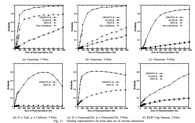
We also test the case where D comes from a distribution other than profile distribution p. Figure 11(d) shows the case where D comes from a 5-dimensional Zipf distribution, but p is a 5-dimensional uniform distribution; Figure 11(e) shows the case where D comes from a Gaussian distribution (σ = 20) and p is Gaussian (σ = 10). It is interesting to observe that using GREEDY-R it is still possible to select from D a limited number of tuples that represent a different distribution p.
Finally, we compared the algorithms using five features extracted from the KDD Cup data. The results (Figure 11(f)) are as expected; GREEDY-R works the best, but due to the dimensionality, HIST-R and RAND-R do not perform as well.
VI. RELATED WORK
Querying Statistical Models: Splash is built on the idea of simultaneously querying profiles (statistical models) and data in a database. A body of related literature describes several other abstractions and systems for incorporating data mining and statistical models into standard or extended SQL.
One recent example is the model-based views of MauveDB [24], which expose interpolated data as a standard relational view. However, we find that this abstraction is not suitable for our system for two reasons: (1) Each model must be declared independently using SQL DDL, which makes adhoc exploration and interactions difficult, and (2) The models themselves are completely hidden behind the interpolated views. More practically, MauveDB provides no API for replacing the underlying statistical models used by the system (e.g., linear interpolation).
Microsoft SQL Server’s DMX [2] and OleDB for DM [41] also integrate data mining models (primarily classification and regression) with standard SQL. However, we also find that this abstraction is not suitable for our purposes because it too requires separate definition of each model and does not allow direct manipulation of models.
IBM DB2 Intelligent Miner [3] supports a variety of data mining tasks, which can be applied to data residing in a relational database. However, to the best of our knowledge, mining models need to be specified one-by-one, either using PMML (a markup language) or the graphical interface.
Exploratory Data Mining: Recent work in exploratory data mining has proposed to view data mining tasks in terms of cube space. For example, Chen et al. proposed the idea of a prediction cube, where classifiers are trained over various data subsets in multidimensional cube space [22]. While this approach is related to our view of statistical models as aggregate functions, to the best of our knowledge, none of the past work has considered integrating cube-based data mining with a relational DBMS or query language.
Representative and Typical Tuples: As part of our system, we also studied the problem of generating “representative” examples to help explain a profile (Section III).
To the best of our knowledge, the problem of explaining a statistical model using a small number of examples has not previously been considered. However, related work has considered various formulations of the following problem: Given a dataset D, produce a “representative” subset thereof, where “representative” is defined in different ways.
Hua et al. considered finding the top-k most “typical” (maximum likelihood) tuples [31]; however, as we showed in Section V-D, the typical tuples often fail our goal of clearly describing the underlying distribution. Liu and Jagadish present a problem formulation based on distance; that is, minimize the distance between the points in D and their representatives [39]. While this approach captures the diversity of data records, it also does not convey the frequency distribution in D. Finally, Pan et al. [42] developed an objective function based on information theory, but it has a different goal from ours in finding a subset from a transactional (itemset) database that simultaneously has high coverage and low redundancy.
Anomaly and Fraud Detection: One of the motivating applications for Splash is ad-hoc log analysis. The idea of anomaly-based intrusion detection goes back to the work of Denning [23]. Typically, however, anomaly detection is viewed as a binary decision (i.e., produce a warning or not), and false positives are often cited as a shortcoming. This provides strong motivation for an ad-hoc query tool in this domain.
Anomaly detection has been studied extensively in operating systems [27], [36], [37], [48], networks (e.g., see recent survey [43]), and for detecting fraud [20], [26]. It is distinct from signature-based intrusion detection (e.g., [4]) which detects pre-defined patterns of abnormal behavior.
Recent work has begun to consider applying anomaly detection to databases. Kamra et al. [33] developed a simple data mining approach, which selects features from the text of SQL queries, and constructs a Naive Bayes classifier to predict the most likely profile (in this case, the RBAC role) for new queries. Other work includes [30], [35], [45], [47].
Auditing for Compliance and Disclosure Control: Recent research has studied the problem of querying the audit logs produced by general-purpose database systems [18], [40]. The interface is usually the following: An auditor specifies a portion of the data in an enterprise database (e.g., Bob’s medical record) using a stylized audit expression. Then, the auditing system is tasked with retrieving all past database queries [18] and sets of queries [40] such that the specified data could have influenced the result. In contrast to this kind of system, which takes a data-centric approach to auditing, when used for log analysis, Splash is behavior-centric.
Tools for auditing disclosure by statistical databases typically aim to detect when successive aggergate queries reveal “too much” about the underlying data, as defined by a disclosure policy [17], [34]. In contrast, when applying Splash to audit logs, our goal is to provide a flexible platform for detecting anomalies in user behavior, rather than detecting disclosure with respect to any particular policy.
VII. CONCLUSION
In this paper, we presented Splash, a novel system supporting ad-hoc simultaneous querying of statistical models and relational data. The fundamental new abstractions supported by Splash are the view of statistical models as aggregation operations, as well as novel operations for interacting with models, including the generation of representative examples. We provided an implementation of Splash, as well as several performance optimizations. Further, an extensive experimental study indicates both that the system scales well, and that the novel abstractions provide a simple alternative to the existing (more complex and rigid) APIs supported by data mining software packages.
REFERENCES
[1] http://www.hhs.gov/ocr/hipaa/.
[2] Data mining extensions (DMX) reference. SQL Server 2005 Books Online. http://technet.microsoft.com.
[3] Db2 intelligent miner. http://www-01.ibm.com/software/data/iminer/.
[4] http://www.snort.org. Retrieved July 16, 2008.
[5] An introduction to computer security: The NIST handbook. NIST Special Publication 800-12.
[6] Kdd cup 1999 dataset. http://archive.ics.uci.edu/ml/ databases/kddcup99/kddcup99.html.
[7] Matlab: The language of technical computing. http://www.mathworks.com/products/matlab/.
[8] Postgresql. http://www.postgresql.org/.
[9] The r project for statistical computing. http://www.r-project.org/.
[10] Result of kdd cup 1999 contest. http://wwwcse.ucsd.edu/ elkan/clresults.html.
[11] Sas: Business intelligence software. http://www.sas.com.
[12] Stata. http://www.stata.com.
[13] Weka 3: Data mining software in java. http://www.cs.waikato.ac.nz/ml/weka/.
[14] Gramm-Leach-Bliley Financial Services Modernization Act, 1999. Pub.L. 106-102, 113 Stat. 1388.
[15] Public Company Accounting Reform and Investor Protection Act of 2002 (Sarbanes-Oxley), 2002. Pub.L. 107-204, 11 Stat. 745.
[16] University of Michigan Health System Compliance Office. Personal communication, 2008.
[17] N. Adam and J. Wortmann. Security-control methods for statistical databases. ACM Computing Surveys, 21(4):515–556, 1989.
[18] R. Agrawal, R. Bayardo, C. Faloutsos, J. Kiernan, R. Rantzau, and R. Srikant. Auditing compliance with a Hippocratic database. In VLDB, 2004.
[19] R. Agrawal, J. Kiernan, R. Srikant, and Y. Xu. Hippocratic databases. In VLDB, 2002.
[20] F. Bonchi, F. Giannotti, G. Mainetto, and D. Pedreschi. A classificationbased methodology for planning audit strategies in fraud detection. In SIGKDD, 1999.
[21] J. Cart. Kaiser fires staffers who snooped into suleman’s files. The Los Angeles Times, March 31 2009.
[22] B. Chen, L. Chen, Y. Lin, and R. Ramakrishnan. Prediction cubes. In VLDB, 2005.
[23] D. Denning. An intrusion-detection model. In IEEE Symposium on Security and Privacy, 1986.
[24] A. Deshpande and S. Madden. MauveDB: Supporting model-based user views in database systems. In SIGMOD, 2006.
[25] P. Dokas, L. Ertoz, V. Kumar, A. Lazarevic, J. Srivastava, and P. Tan. Data mining for network intrusion detection. In Proceedings of NSF Workshop on Next Generation Data Mining, 2002.
[26] T. Fawcett and F. Provost. Adaptive fraud detection. Data Mining and Knowledge Discovery, 1, 1997.
[27] S. Forrest, S. Hofmeyr, A. Somayaji, and T. Longstaff. A sense of self for UNIX processes. In IEEE Symposium on Security and Privacy, 1996.
[28] J. Gray, S.Chaudhuri, A. Bosworth, A. Layman, D. Reichart, M. Venkatrao, F. Pellow, and H. Pirahesh. Data cube: A relational aggregation operator generalizing group-by, cross-tab, and sub-totals. Data Mining and Knowledge Discovery, 1(1), 1996.
[29] V. Harinarayan, A. Rajaraman, and J. Ullman. Implementing data cube efficiently. In SIGMOD, 1996.
[30] Y. Hu and B. Panda. Identification of malicious transactions in database systems. In IDEAS, 2003.
[31] M. Hua, J. Pei, A. Fu, X. Lin, and H. Leung. Efficiently answering top-k typicality queries. In VLDB, 2007.
[32] Y. Ioannidis and Y. Poosala. Balancing histogram optimality and practicality for query result size estimation. In SIGMOD, 1995.
[33] A. Kamra, E. Terzi, and E. Bertino. Detecting anomalous access patterns in relational databases. VLDB Journal, 2007.
[34] K. Kenthapadi, N. Mishra, and K. Nissim. Simulatable auditing. In PODS, 2005.
[35] C. Kruegel and G. Vigna. Anomaly detection of web-based attacks. In ACM Conference on Computer and Communications Security, 2003.
[36] W. Lee and S. Stolfo. Learning patterns from unix process execution traces for intrusion detection. In AAAI Workshop on AI Methods in Fraud and Risk Management, 1997.
[37] W. Lee and S. Stolfo. Data mining approaches for intrusion detection. In USENIX Security Symposium, 1998.
[38] W. Lee, S. Stolfo, and K. Mok. A data mining framework for building intrusion detection models. In Proceedings of IEEE Symposium on Security and Privacy, Oakland, 1999.
[39] B. Liu and H. Jagadish. Using trees to depict a forest. In VLDB, 2009.
[40] R. Motwani, S. Nabar, and D. Thomas. Auditing sql queries. In ICDE, 2008.
[41] A. Netz, S. Chaudhuri, U. Fayyad, and J. Bernhardt. Integrating data mining with SQL databases: OLE DB for data mining. In ICDE, 2001.
[42] F. Pan, W. Wang, A. Tung, and J. Yang. Finding representative set from massive data. In ICDM, 2005.
[43] A. Patcha and J. Park. An overview of anomaly detection techniques: Existing solutions and latest technological trends. Computer Networks, 51:3448–3470, 2007.
[44] Y. Poosala and Y. Ioannidis. Selectivity estimation without the attribute value independence assumption. In VLDB, 1997.
[45] A. Spalka and J. Lehnhardt. A comprehensive approach to anomaly detection in relational databases. In Proceedings of the 19th IFIP WG 11.3 Working Conference on Data and Applications Security, 2005.
[46] E. Tombini, H. Debar, L. Me, and M. Ducasse. A serial combination of anomly and misuse idses applied to http traffic. In Computer Security Applications Conference, 2004.
[47] F. Valeur, D. Mutz, and G. Vigna. A learning-based approach to the detection of SQL attacks. In International Conference on Detection of Intrusions and Malware, and Vulnerability Assessment, 2003.
[48] C. Warrender, S. Forrest, and B. Pearlmutter. Detecting intrusions using system calls: Alternative data models. In IEEE Symposium on Security and Privacy, 1999.
[49] J. Zhang and M. Zulkernine. A hybrid network intrusion detection technique using random forests. In First International Conference on Availability, Reliability and Security, 2006.
[50] Y. Zhang, H. Herodotou, and J. Yang. Riot: I/o-efficient numerical computing without sql. In CIDR, 2009.
1We will use capital letters X1, .., Xn, P to denote feature/attribute names, and lower-case letters x, p, etc. to denote values.

2 In practice, we expect a combination of discrete and continuous features; the generalization is straightforward.

3This is closely related to the Naive Bayes assumption.

4Of course, KL-divergence is not symmetric, so a common trick computes both values and takes the average.

5Suppose that a space partitioning algorithm divides the space into l subregions {R1, R2, ..., Rl}. For the region Ri (1 ≤ i ≤ l), we need to pick k ∗ R Ri p points as representatives for that region.

6 Interestingly, the current interface for user-defined aggregation in PostgreSQL does not reflect the size of the aggregation results (i.e., a large profile object as opposed to an integer). However, we expect that a simple addition to the interface would provide the optimizer with better information, allowing it to choose hashing vs. sorting.
Author: Lujun Fang, Kristen LeFevre